
www.TestsTestsTests.com

Pivot Tables Excel Tutorial
Excel 2010 Training –
Working with Data
Free Online Microsoft Excel Tutorial
* What is a Pivot Table?
*
Inserting a Pivot Table
* Pivot Table Fields
* Using a Report Filter
By moving the data Pivot Tables let you organize, analyze and summarize large amounts of data in lots of different ways.
Test your Excel skills with the corresponding FREE Online Multiple Choice
Pivot Tables Excel Test
* What is a Pivot Table?
A Pivot Table is a fancy name for a data analysis tool that allows you to create a summary or report based on an information source. Pivot tables are highly manipulatable and quick to create. In Excel, the Pivot Table function has numerous add-on options for quickly creating data sets and reports with literally numerous variations.
So what does a Pivot Table look like?
Study the screenshot below for an image of a Pivot Table:

The data area is the data that has been organized into a table.
On the left-hand side of the image, the PivotTable Field List contains the tools that can be used to manipulate which data is analyzed and how it is displayed.
The greatest benefit of using Pivot Tables is that you can quickly change how data is analyzed and what information is displayed.
In the screenshot below, by changing one setting, the report is now displaying values for each product as percentages of the total sales of all products:

In essence, Pivot Tables turn your static data into dynamic data that can be manipulated to provide an analysis of information from every possible angle.
To carry out the functions which are built into Pivot Tables, will require several regular Excel worksheets and multiple formulas, to recreate.
* Inserting a Pivot Table
Working with Pivot Tables may appear daunting when you start as it takes a little while to adjust to the different functions and analysis tools. Many people give up on using Pivot Tables far too early and it is worth investing time in practicing how to insert a Pivot Table.
1. A Pivot Table is an analysis tool used to analyze existing data. You cannot start a Pivot Table based on zero data. So the first step would be to find or create a worksheet containing multiple labelled rows and columns of populated cells.
2. Select the data range (rows and columns) in the worksheet that you wish to analyze. Do not select a worksheet heading.
3. Click on the Insert tab on the Ribbon.
4. In the Tables group, click on Pivot Table and select Pivot Table from the list.
5. In the Create Pivot Table dialogue box, the Select a Table or Range and New Worksheet radio buttons should be selected by default. Study the screenshot below to ensure you are still on the right track:

6. Press OK to create the Pivot Table.
The Pivot Table will be inserted on a new worksheet (based on the selections above). The Pivot Area will be blank until data labels for columns, rows and filters are selected. Although this sounds intimidating, hang in there, these are really just dragging and dropping your column and row labels into specific areas of the PivotTable Field List.
Before any labels are selected, your Pivot Table worksheet display will be similar to the screenshot below:
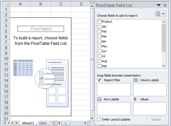
Depending on the data contained in the worksheet on which you are basing the Pivot Table, these labels will appear in the PivotTable Field list.
To access the PivotTable Options and Field list, you need to click in the Pivot Table area. If you click away from the Pivot Table area, you will note the PivotTable Field list and other Pivot Table options, disappear.
The Pivot Table contextual tab containing Pivot Table Tools for Design and Options, will also only be available when the Pivot Table area is selected. In the screenshot below, these contextual tabs are displayed and circled in yellow:

Experiment with clicking in the Pivot Table area and away and take note of the options that appear and disappear when you do this.
In the next section of this tutorial we look at how to set-up the Pivot Table by organizing the fields.
* Pivot Table Fields
In essence, Pivot Table fields are the row and column labels of the data that you selected to base the Pivot Table on as well as all the data contained within this selection.
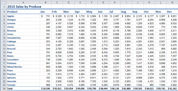
For example, the screenshot below contains row labels with product/produce names such as Apples, Oranges, etc. The column labels are the months of the year and the data shows the total sales for each product/produce for that month.
The total row at the bottom of the data shows the total sales for each month of all products:
To use Pivot Table Fields it is important to first understand the data you want to base the Pivot Table on.
Next, you need to decide what information you want to analyze using the Pivot Table function.
In our example screenshot above, we may, for example, wish to analyze the percentage of sales that each product’s monthly sale contributes to all sales.
To analyze this data:
1. Ensure the PivotTable Field List options are displayed on the left hand side. You have to insert a Pivot Table first (see instructions in the previous section above) and click in the Pivot Table area for these options to be available.
2. Decide which data set you want to use for the Row and Column labels. For our example, we want to show the percentage of the total that each product’s monthly sale makes up of the whole.
3. In the PivotTable Field List, drag the column and row labels into the Report Filter, Column Labels, Row Labels and Values boxes. Don’t be alarmed at how your data will change or be displayed, you can keep dragging labels into, out of, or between these boxes to view the data in different ways.
4. Study the screenshot below. To analyze the percentages of the whole that each product makes up, we dragged the column heading Product into the Row Labels box. The column headings for each month were selected and dragged into the Values box as we wish to analyze the totals for each month.

5. Finally, to change the values to percentages, click on Options in the PivotTable Tools contextual tab.
6. In the Calculations group, select Show Value As and select an option from the list. Selecting % of Grand Total will show each product’s monthly sale as a percentage of the total sales of all products.
The above is just one simple example of what can be achieved using the Pivot Table reporting tool. It is worth looking through all the available options and experimenting with analyzing data using different calculation types in the Values box, switching Column and Row labels around and changing settings.
* Using a Report Filter
Report filters are a functional mixture between the regular Find and Replace function and Data Filters in Excel. Using a Report Filter, you can create a data finder on the same sheet on which data is contained or on a separate worksheet. This is useful if you frequently need to look up information in a worksheet.
To create a Report Filter:
1. Decide what you wish to filter the data for and which column label represents this data.
2. Insert a Pivot Table by selecting all the data you require to be included in the filter, clicking on the Insert tab on the Ribbon and selecting Insert Pivot Table.
3. In the PivotTable Field List, drag the column label for the items you wish to filter by, into the Report Filter box.
4. Drag to labels containing the values you wish to filter by, into the Values box.
In the example below, we have created a simple filter which we can use to look at individual or selections of products and the total revenue for each:

To use the filter to look up items:
1. Click on the dropdown arrow next to the filter in the worksheet (circled in yellow in the screenshot above).
2. Select the individual item in the list to filter by, or, select multiple items by ticking the Select Multiple Items checkbox and then checking the boxes for the items to include in the filter:

3. Click OK to accept the variables and display the filter results.
Pivot Tables are incredibly complex and powerful tools. The best way to learn about them is to experiment with the different options and of course to keep doing Excel Tutorials and Quizzes!
Now you have done the tutorial…
Test your Excel skills with the corresponding FREE Online Multiple Choice
Pivot Tables Excel Test