www.TestsTestsTests.com
Formatting Text In Excel –
Formatting Numbers Excel Tutorial
Excel 2016 Tutorial
Data Entry & Formatting in Excel Lesson
Free Online Microsoft Excel Tutorial
* Selecting a font type, color and size in Excel 2016
* Using bold, italic and underline
* Selecting and applying built-in cell styles in Excel
* Using the format painter
Excel 2016
* Excel clear formatting from cells
|
Formatting functions in Excel provide options that will make the data in your worksheet easier to read and understand. Use different fonts, font colors and sizes, bold, italic, underline and built in styles to create visually appealing worksheets. |
 |
* Selecting a font type, color and size in Excel 2016
Formatting text and numbers in Excel by changing the font type and the text size, can make a worksheet not only look neat, but can also make it easier to read.
The example below is a worksheet with no formatting applied:
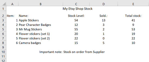
To change the font of the heading “My Etsy Shop Stock”, do the following:
1. Click the cell containing the text you want to change the font for (in our example this is the merged cell in Row 1.
2. Under the Home tab on the Ribbon, in the Font group, click the dropdown arrow next to the font box (outlined in the orange box in the screenshot below).
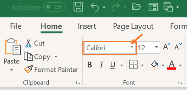
3. From the font dropdown list, select a font that you like and click on it to apply it to the selected cell.
TIP: you can change the font as many times as you want! Use the Undo button to return to a previous applied font. You can download and install many fun and professional fonts from the Internet. Do a Google search to find some and use them in your Excel 2016 workbooks.
To change font size:
1. Select the cell or cells containing the text/numbers you want to change the size of.
2. Under the Home tab on the Ribbon, in the Font group, either:
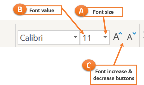
A. Click on the dropdown Font Size arrow next to the Font Value box and select a larger sized font by clicking a higher number value, e.g. a font size of 45 is bigger than one of 12.
B. Type a number value for the font size you want directly into the Font Value box and press the Enter key on your keyboard
C. Use the Increase and Decrease Font buttons in the Font group to make the font smaller or larger
To change the font color:
1. Select the cell or cells containing the text/numbers you want to change the color of.
2. Under the Home tab on the Ribbon, in the Font group, click on the dropdown arrow next to the color button and select the color you wish to apply.
Our worksheet example now has new fonts, font color and size changes applied and looks like this:
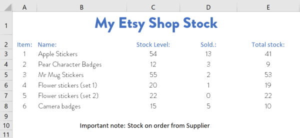
Compare the above screenshot to the one we started with – I’m sure you’ll agree the new font type, color and size options applied makes a huge difference!
* Using Bold, Italic and Underline
The Bold, Italic and Underline functions in Excel allows you to quickly add emphasis to text and numbers.To apply Bold, Italic or Underline to text:
1. Select the cell(s) containing the text or even a portion of the text, like a single word, that you want to apply either Bold, Italic or Underline formatting to.
2. Click on the Home tab on the Ribbon, and in the Font group, select Bold, Italic and/or underline. The formatting will immediately be applied to the selected text/numbers.
TIP: Use the following shortcut keys to apply Bold, Italic and/or Underline to selected text/numbers:
Bold: Ctrl + B
Italic: Ctrl + I
Underline: Ctrl + U
Go ahead and experiment with applying Bold, Italic and Underline using the shortcut key combinations.
* Selecting and applying built-in cell styles in Excel
Excel 2016 has a built in Cell Style gallery that allows you to pick a formatting combination that you like and apply it to your worksheet. This is a great timesaver as instead of trying endless font type, size and color combinations, you can instantly apply a great looking format. Let’s look at how to do this!
1. Select the cells that you want to format, for example, the cell containing the heading of the worksheet.
2. Under the Home tab on the Ribbon, in the Styles group, click on the Cell Styles button (outlined in orange in the screenshot below.
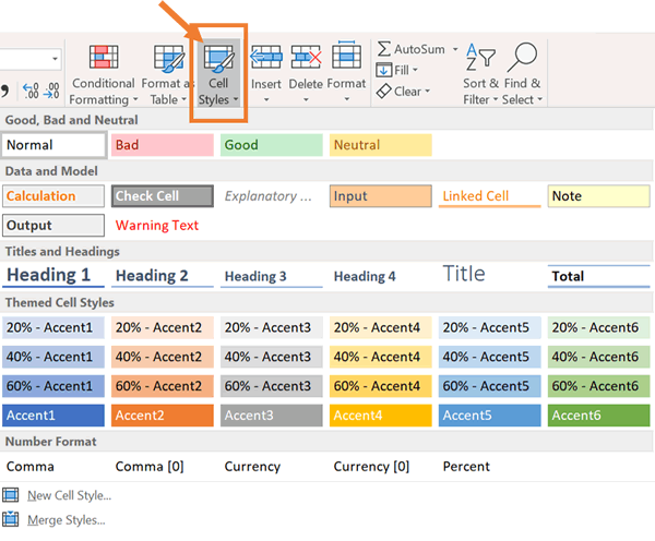
3. From the Cell Styles gallery (see screenshot above), hover over the heading styles to see what it will look like when applied and click on the style you like to apply it. If you don’t like the style you selected, simply select another one which will automatically replace the last style you selected.
You can also create your own styles:
1. Format a cell using the font type, font size, bold, italic and underline functions described earlier in this tutorial.
2. With the formatted cell selected, go to the Cell Styles gallery (which you’ll find under the Home tab on the Ribbon in the Styles group).
3. Click on the New Cell Style option that you’ll find at the bottom of the Cell Styles gallery. This will launch the Style dialog box.
4. Give your style a meaningful name and click OK.
5. Go back into the Cell Styles gallery and you’ll see the style you created is now available to select from the top row of the gallery.
TIP: Creating multiple cell styles will help you to quickly format your worksheet and other worksheets within your Excel workbook.
* Using the format painter Excel 2016
The Format Painter is an amazing and magical tool in all Microsoft Office programs. You use the Format Painter to replicate formatting from one cell to another with the click of a button. Sounds too good to be true? Let’s look at how to use this function.
1. Select a cell that contains the formatting that you want to replicate to other cells.
2. Under the Home tab on the Ribbon in the Clipboard group, you will find the Format Painter – see outlined in orange in the screenshot below:
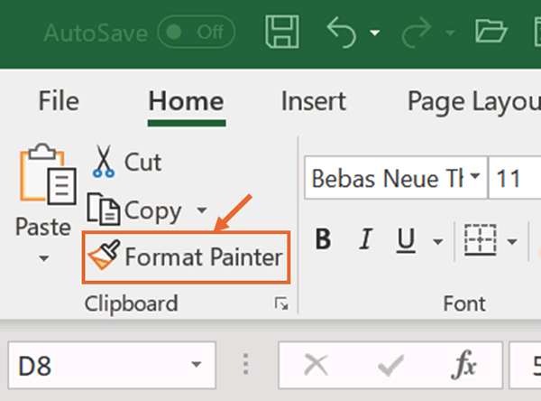
Click the format painter button – you will notice that your cursor has changes into a tiny little roller paint brush.
3. Finally, click the cell you want to apply the formatting to, to apply it.
TIP: If you double click the Format Painter icon (see outlined in orange in the screenshot above) you can continue painting as many cells as you wish. Press the escape key to deselect the Format Painter.
* Excel clear formatting from cells
In this tutorial we’ve spent some time looking at how to apply formatting such as fonts, font styles, colors, bold, italic, underline and how to replicate formatting. In this final part of the tutorial we will look at how to quickly remove all formatting.
It is easy to fall into the trap of thinking that you need to remove formatting manually or using the Undo button, but there is a much quicker way to achieve this.
1. Select the cell(s) or entire worksheet you wish to remove the formatting from.
2. Under the Home tab on the Ribbon, in the Editing group, click on the dropdown arrow next to the Clear button (outlined in orange in the screenshot below).
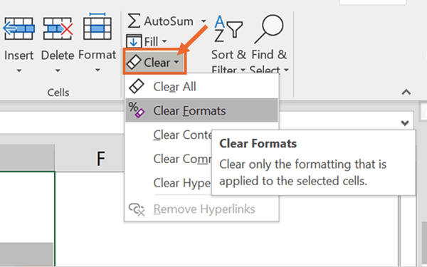
3. Select the Clear Formatting option by clicking on it. All the formatting in your selected cells will instantly be removed.
Woohoo! Now that you have done the tutorial:
Test your Excel skills with the corresponding FREE Online Multiple Choice
Formatting Text and Numbers in Excel – Data Entry and Formatting
TRY THE NEXT TUTORIAL: Aligning Cell Content in Excel 2016 Tutorial
TRY THE NEXT TEST: Aligning Cell Content in Excel 2016 Test


