
www.TestsTestsTests.com

Basic Worksheet Formatting Tutorial
Free Online Microsoft Excel Tutorial
Excel 2010 –
Worksheets
* Inserting & Deleting Cells, Rows & Columns
*
Setting Width & Height for Columns & Rows
*
Inserting & Formatting Borders
*
Inserting Headers, Footers & Page Numbers
Making your worksheets easy to read and understand is crucial. Formatting is the key. This includes changing the appearance of the worksheet including inserting and deleting columns and rows, changing column widths and row heights, cell color and borders and how to add Headers, Footers and page numbers.
Test your Excel skills with the corresponding FREE Online Multiple Choice
Excel Basic Worksheet Formatting Test
* Inserting and Deleting Cells, Rows and Columns
Examining a worksheet in Excel, the first thing you probably notice is the grid that fills most of the Excel screen. This grid is made up of multiple columns and rows and any data you add to a worksheet will be contained in separate cells, rows and columns. It is therefore essential that you are comfortable with inserting and deleting cells, rows and columns in Excel.
To insert a cell:
1. Position your cursor in the cell currently occupying the space on your worksheet where you wish to insert a new cell.
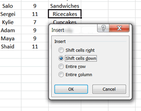
2. On the Home Tab in the Cells group, click on the Insert Button. Another method is to right-click the cell where you wish to insert a new cell and select Insert from the menu list. This will open the Insert dialogue box (see screenshot below). Tick the: Shift Cells Down or Shift Cells Right buttons depending on where you wish to insert the blank cell.
3. A blank cell will be inserted in the position you selected and the selected cell will move to a new position (down or right).
To insert a column:
1. Select the column immediately to the right of where you wish to insert a new column by clicking on the column label (column labels are the letters of the alphabet shaded in grey at the top of the grid) to select the whole column.
2. Right-click on the selected column and select Insert from the menu list.
3. This will insert a blank column to the left of the column you selected.
To insert a row:
1. Select the row above which you wish to insert a new row by clicking on the row label (row labels are the grey shaded numbers running alongside the left margin of the grid) to select the whole row.
2. Right-click on the selected row and select Insert from the menu list.
3. This will insert a blank row above the row you have selected.
TIP: To insert multiple cells, rows or columns, select the number of cells, rows or columns you wish to insert before clicking on the Insert button. For example, if you select three rows, Excel will insert three blank rows above your selection when you right click the selection and then on Insert in the menu list.
Being able to delete cells, rows and columns, is just as important as being able to insert them.
To delete a cell or multiple cells:
1. Select the cell to delete, right-click the cell and select Delete from the menu list.
2. The Delete dialogue box will appear from where you need to make a selection between shifting the cells below the deleted cell upwards, or shifting the cells to the right of the deleted cell, to the left.
3. Delete multiple cells by first selecting cells by dragging through them with your mouse or select non-adjacent cells by holding down the Ctrl key on your keyboard whilst selecting cells, right-click the selection and then click on Delete in the menu list.
To delete a column or multiple columns:
1. Select the column to delete, right click the selected column and select Delete from the menu list.
2. The column will be deleted.
3. Delete multiple columns by selecting and dragging through the column labels with your mouse or select non-adjacent columns by holding down the Ctrl key on your keyboard whilst selecting columns then right-click the selection and then click on Delete in the menu list.
To delete a row or multiple rows:
1. Select the row to delete, right click the selected row and select Delete from the menu list.
2. The row will be deleted.
3. Delete multiple rows by selecting and dragging through the row labels with your mouse or select non-adjacent rows by holding down the Ctrl key on your keyboard whilst selecting rows then right-click the selection and then click on Delete in the menu list.
* Setting Width and Height for Columns and Rows
Worksheets can be difficult to read. Rows and columns that are too close together or too far apart may look chaotic, crowded or take up too much space. Setting width and height parameters for rows and columns can make an enormous difference in the readability and overall look of a worksheet.
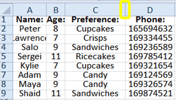
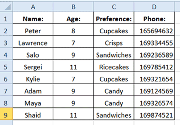
Examine the screenshot below. This is just a very simple worksheet, but it is clear the data is cramped together. It is hard to read and is aesthetically unpleasing.
To change column width:
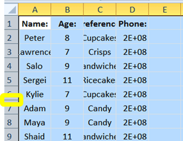
1. Move either the right or left column divider line (circled in yellow in the screenshot above) by clicking on it and dragging it to make the column wider or narrower.
2. Double clicking the divider line will automatically resize the column to fit the contents.
3. Selecting multiple columns or the whole worksheet and double-clicking the divider line between any of the selected columns, will automatically resize all columns to fit the contents.
4. Selecting multiple columns and dragging the divider line between any of the selected columns will automatically resize all columns to be the same size as the column whose divider you are dragging.
To change row height:
1. Move either the top or bottom divider line (circled in yellow in the screenshot below) by clicking on it and dragging it upwards or downwards to change the height of a row.
2. Double clicking the divider line will automatically resize the row height to fit the contents.
3. Selecting multiple rows or the whole worksheet and double-clicking the divider line between any of the selected rows, will automatically resize all rows to fit the contents.
4. Selecting multiple rows and dragging the divider line between any of the selected rows will automatically resize all rows to be the same size as the row whose divider you are dragging.
The above is the most frequently used and convenient methods for changing row height and column width. For more options or to set precise width and height values:
1. Under the Home tab on the Ribbon, in the Cells group, click on the Format button.
2. From the Format menu select either Row Height or Column Width to insert exact sizes for these.
* Inserting and Formatting Borders
Borders make worksheets easier to read. You can use borders to outline data, emphasize important cells, rows or columns or simply to make the worksheet easier to read, especially when it is printed.
First decide where you would like borders for your worksheet to appear.
To add borders to a worksheet:
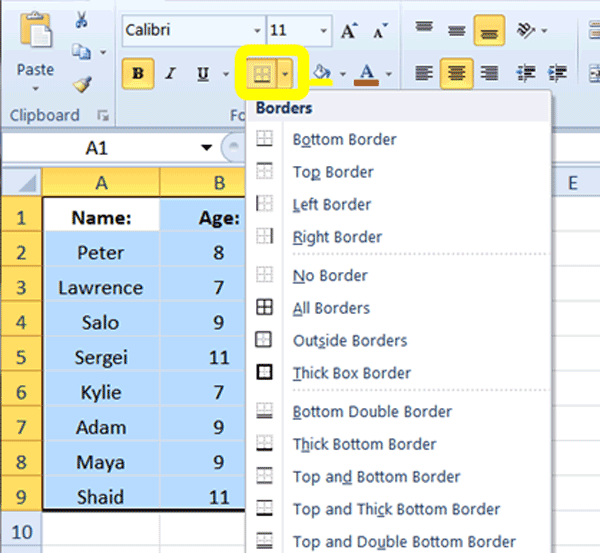
1. Select the rows, columns or cells you wish to apply borders to.
2. Under the Home tab in the Font group, click on the dropdown arrow next to the Border button (circled in yellow in the screenshot below) to view the list of available border types:
3. It is worth experimenting with the various border options. The most often used borders is the All Borders option, which adds borderlines throughout your selected cells, columns and rows or the Outside Borders option, which places a border around the outside of your selected cells, columns and rows.
This is an example of All Borders that has been applied to a selected cell range:
This is an example of Outside Borders that has been applied to a selected cell range:
Equally as important as knowing how to apply borders to a worksheet, is knowing how to remove borders.
To remove all borders from a cell range:
1. Select the cell range you wish to remove all borders from.
2. Click on the dropdown arrow next to the Borders button in the Font group under the Home tab,
3. Select No Border from the list of border types to remove all borders from the selected cells.
Borders can be any color and you can even set a style for the lines of your borders to really emphasize sections of data or to round off your worksheet.
To change the color and/or style of borders:
1. Select the cell range to which you wish to apply the border color and/or style.
2. Click on the dropdown arrow next to the Border button in the Font group under the Home tab and select More Borders from the list of options.
3. This will launch the Format Cells dialogue box (see screenshot below). Ensure the Border tab is selected:
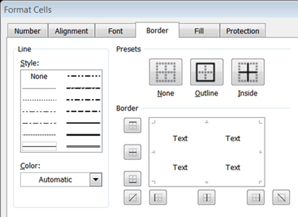
4. First pick a Style for your borders by selecting one of the line types in the Style box.
5. Next set the color for your borders by picking a color from the Color dropdown list or leave it on Automatic to select the default line color for your worksheet.
6. The final step is to apply your borders. You can do this by clicking on one of the Presets in the Format Cells dialogue box or by clicking on individual lines in the Border area. The preview screen with the four boxes labelled text will display what the border style, colors and lines will look like when applied.
7. Once you are happy with the look of your borders, click on OK to apply to your worksheet.
8. To edit borders once applied, you can click back on the More Borders option in the Borders list in the Font group.
9. To remove borders, click on the No Border button in the Borders list.
* Inserting Headers, Footers and Page Numbers
Headers, footers and page numbers all work together to make a worksheet look professional and helps with collating printed worksheets. Adding these elements to a worksheet can also save you time and with the busy schedules most of us manage, any tools for saving time are essential.
Headers are inserted into the top margin of a worksheet and may contain elements such as text, images, page numbers, tables and formatting. Headers are automatically repeated in the same area of the top margin of all pages in a worksheet when printed.
To insert a Header into a worksheet:
1. Click on the Insert tab on the Ribbon. In the Text group, click on the Header & Footer button.
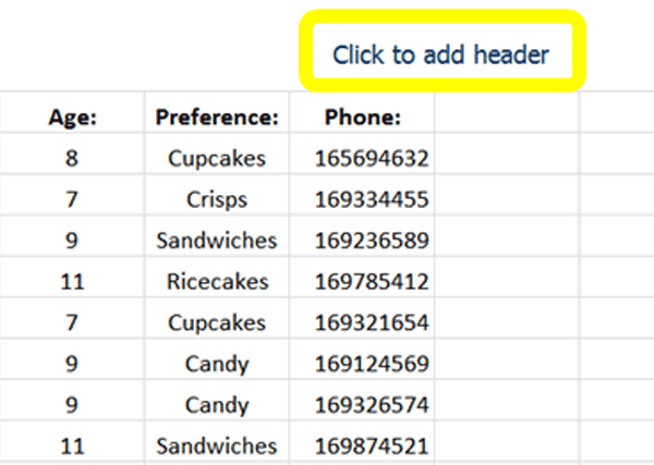
2. Click in the area on your worksheet labelled: Click to add header (circled in yellow in the screenshot below):
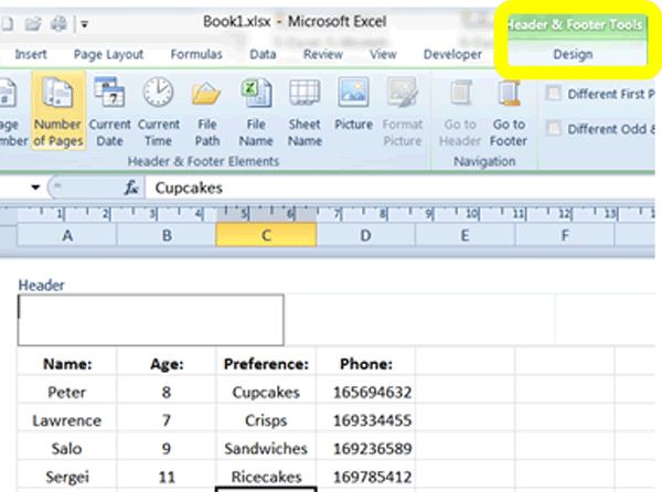
3. When you click in the Header area, the Header & Footer Tools tab will appear above the Ribbon. To access tools and options for the Header area, click on the Design tab (circled in yellow in the screenshot below). This tab will only be available after you have clicked in the Header (or Footer) area. You will not have access to this set of options without clicking the Header (or Footer) area.
4. You can type directly into the Header area by clicking in the left, center or right box and typing the text you wish to appear at the top of every page when your worksheet is printed.
5. Use the options available from the Header & Footer Tools – Design menu to insert any of the elements in the Header & Footer Elements group, such as Page Numbers, Time, Date or Pictures.
Footers are the same as Headers but appear at the bottom of a page when the worksheet is printed.
To insert a Footer:
1. Click on the Insert tab on the Ribbon. In the Text group, click on the Header & Footer button.
2. Scroll to the bottom of the page and click in the area labelled: Click to add footer.
3. When you click in the footer area, the Header & Footer Tools Design tab will appear on the Ribbon. To access tools and options for the Footer area, click on the Design tab. This tab will only be available after you have clicked in the Footer (or Header) area. You will not have access to this set of options without clicking the Header (or Footer) area.
4. You can type directly into the Footer area by clicking in the left, center or right box and typing the text you wish to appear at the bottom of every page when your worksheet is printed.
5. Use the options available from the Header & Footer Tools – Design menu to insert any of the elements in the Header & Footer Elements group, such as Page Numbers, Time, Date or Pictures.
Headers & Footers can be formatted using normal formatting tools such as font and paragraph settings.
* To delete Headers & Footers:
1. Click on the Insert tab and in the Text group, click on the Header & Footer button.
2. Click in either the Header or Footer region of your document to activate the Header & Footer Tools – Design tab.
3. Click on the Design tab and in the Header & Footer group click either on Header or Footer (depending on which one you wish to delete) and select None from the menu. This will remove all the content in either the Header or Footer region.
To return to the Normal worksheet view when you are done editing your Headers and Footers:
1. Click on the View tab on the Ribbon.
2. In the Worksheet Views group, click on Normal. This will return the view to the default view where you can continue to work in your worksheet.
Headers & Footers will not display in the Normal View. To view Headers & Footers you must be in the Page Layout View or Print Preview panel.
To insert Page Numbers:
1. Click on the Insert tab on the Ribbon. In the Text group, click on the Header & Footer button.
2. Click where you wish to insert the page number: the Header or Footer area and the position (left, center or right),
3. Ensure the Header & Footer Tools – Design tab is activated by clicking on it to launch the Header & Footer options.
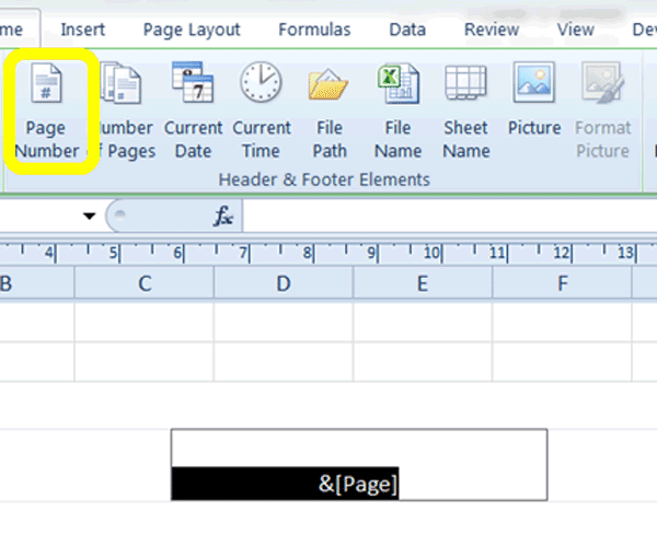
4. In the Header & Footer Elements group, click on the Page Number button (circled in yellow in the screenshot below) to number the pages of your document. This will insert the code: &[Page] into the space, but when you click back in the body of the document, the page number will be visible:
5. To delete page numbers, use the same procedure as for deleting Headers & Footers or simply click in the Header or Footer area containing the page number, select the contents and press Delete on your keyboard.
Experiment with creating different content in the Header & Footer regions of a worksheet. For example, add a company name or logo, the worksheet name and page numbers. Use Print Preview (Ctrl+P) to view what the Header & Footers will look like when printed.