www.TestsTestsTests.com
Using Data Outline Tools Tutorial
Excel 2010 Training –
Working with Data
Free Online Microsoft Excel Tutorial
* Creating an Outline
*
Viewing Sections of an Outline
* Inserting Subtotals
* Clearing an Outline
When analyzing worksheets containing multiple rows of data and different categories it can be difficult to get a quick overview of data. Outline tools such as Group and Subtotal give you quick results when looking for answers in your data.
Test your Excel skills with the corresponding FREE Online Multiple Choice
Using Data Outline Tools Excel Test
* Creating an Outline
The Outline function in Excel provides a quick and simple way to organize data. Outlines organize data into groups according to set levels and provide buttons with the functionality to collapse or expand these groups. Each worksheet can have a maximum of eight outline levels, which is more than most Excel users will ever need. You use the Group function to create outlines of data.
Study the screenshot below:
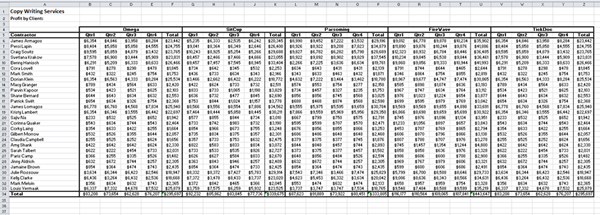
This is a large worksheet organized by the profits of each contractor, firstly by company and secondly by quarter. To view and compare data in a worksheet this size will require much scrolling to the right and back to the left in order to view the totals for relevant levels and to compare them.
The Outline function is ideal in this type of scenario as it allows you to create a quick summary of data based on levels.
To apply an outline to a worksheet:
1. Open the worksheet you wish to apply the outline to.
2. Select the cell ranges you wish to organize into an outline. (To quickly select a cell range, select the first cell in the range, hold down the Shift key on your keyboard and select the last cell in the range.)
3. Click on the Data tab on the Ribbon and in the Outline group, click on the Group button.
4. Next, click on Auto Outline. This will add row-level and column-level selectors or symbols and collapse or expand buttons (depending on the data selected).
The next section deals with how to use the row– and column-level selector symbols and the collapse and expand buttons.
* Viewing Sections of an Outline
When an Outline is applied to a worksheet, it may at first appear as if parts of the worksheet are hidden. It may also be your experience that the outline symbols and lines at the top of columns, on the side of rows and at the corner of the worksheet result in the data appearing more confusing than without the Outline applied!You are not alone if this is your experience. The Outline function view takes a little bit of getting used to and armed with the knowledge of what all the Outline indicators do, you will become a master at creating data summaries in no time!
To navigate and manage the Outline view it is important to know what the symbols/buttons and/or selectors’ functions are:
1. The collapse symbol resembles a minus sign and is used to collapse sections of an outline so that only totals are displayed.
Study the screenshot below:
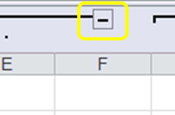
The minus symbol circled in yellow above, is called the collapse symbol or button. When you click this, the area of the worksheet it controls, will be minimized.
You will note that after pressing the collapse symbol and minimizing a section, the symbol changes into an expand symbol.
2. The expand symbol resembles a plus sign and is used to expand sections of an outline so that all the rows or columns (as applicable) for that section are displayed.
Study the screenshot below:
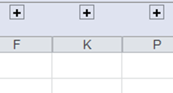
The plus symbols at the top of these columns are known as expand symbols or buttons. When you click an expand button, the section that has been collapsed will be maximized again displaying all the columns or rows (whichever is applicable) for that section of the outline.
Once you click an expand button and the section is expanded, it will change back to a collapse button (the minus symbol).
3. In addition to using the collapse and expand buttons to view or hide sections of the outline, you can also use the level buttons to show or hide entire levels of the worksheet. You will use these if you wish to collapse or expand ALL the sections at a certain level.
Study the screenshot below:
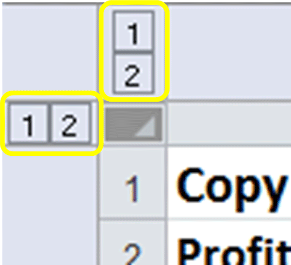
The symbols circled in yellow above indicate that an outline has been applied to this worksheet at a column and row level.
Clicking on the 1 in the screenshot above, at either row or column level, will collapse all the data at this level in the worksheet. You can have up to eight levels in a worksheet. You create levels by selecting sections of data and creating new outlines for different levels of data. For example, you can have a worksheet that has one level for each year, a second level for each quarter and perhaps a third level for each month.
Clicking on the 2 in the screenshot above, at either row or column level, will expand all the data at this level in the worksheet.
When you have multiple levels, you can use the expand and collapse buttons to display or hide specific levels only. This is a great way to quickly have a summary at hand of vast amounts of data.
* Inserting Subtotals
The Subtotal function in Excel is like AutoSum on steroids. Instead of spending your much deserved coffee break inserting formulas and rows into a worksheet, use the Subtotal function to quickly do all the hard work for you.
The Subtotal function can be used to determine the sum, product, count, average, max, min and other calculations, of sections.
Study the section of a worksheet in the screenshot below:
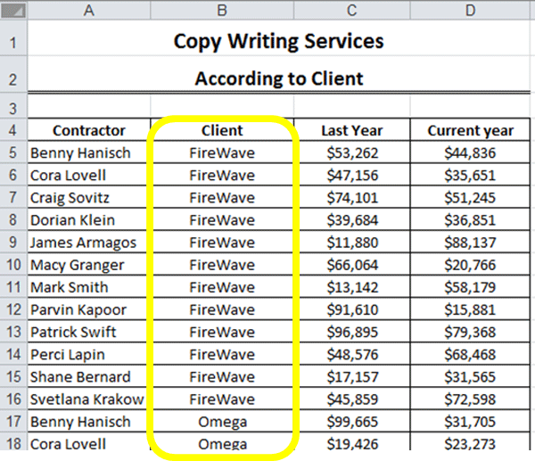
In this worksheet, the year on year profits generated by each contractor per client is displayed. The worksheet is sorted according to clients (with clients grouped together).
To use the Subtotal function:
1. Open the worksheet containing the data you wish to summarize using Subtotal.
2. Ensure the data is sorted according to the criteria you wish to subtotal it. For example, to display subtotals per client, we would ensure the worksheet is sorted so that all the same clients are together (as per the screenshot above).
In contrast, to display a subtotal for each contractor, we would sort the worksheet so that all instances of the same contractor are grouped together (see screenshot below):
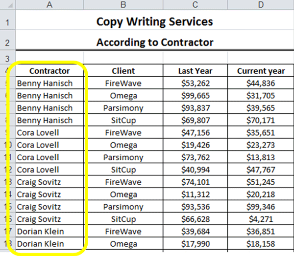
3. Select the cell range, including headings, you wish to organize using the Subtotal function.
4. Click on the Data tab on the Ribbon. In the Outline group, click on the Subtotal button. This will launch the Subtotal dialog box:
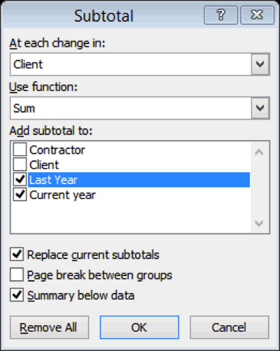
5. In the first box, under the At Each Change in heading, select the heading that represents the group of numbers you wish to apply the Subtotal to. For example, in our worksheet we could total the last and current year totals for each client or for each contractor.
6. Select the function you wish to use in the Subtotal, for example, Sum.
7. Select which column to add the Subtotal to. In the example above, the Subtotal will be inserted for each client in the columns titled: Last Year and Current Year.
8. Tick the option boxes for replacing current subtotals, inserting a page break or inserting a summary below the data. This will depend on how you wish the Subtotals and groupings to display and it is worth experimenting with different options.
9. Press OK to apply the subtotals.
Based on the selections made in the Subtotal dialog box above, the data with subtotals will display as follows (see screenshot below):

The areas circled in yellow in the screenshot above are the subtotals which the Subtotal function has inserted based on the selections made in the Subtotal dialog box.
You will also note that the usual outline buttons are also displayed. You can use these to expand or collapse sections to view subtotals only or all the data in the worksheet.
* Clearing an Outline
Outlines are often used to only temporarily apply summaries to data for analytical purposes. To quickly remove all outlines and return the data to the pre-outline view, we use the Ungroup function.
To clear outlines:
1. Open the worksheet containing the outlined data.
2. Click on the Data tab on the Ribbon.
3. In the Outlines group, click on Ungroup and select Clear Outline (highlighted in yellow in the screenshot below):
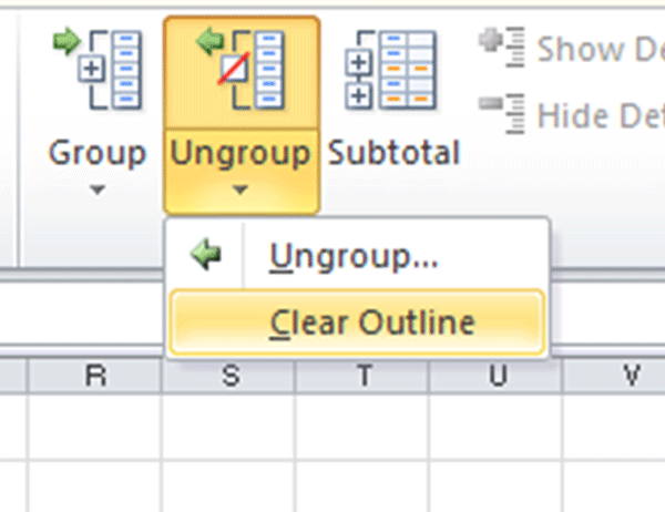
All outlines applied to the worksheet will be removed and your worksheet will be returned to its pre-outline status.
Note that subtotals will not be removed when using the Clear Outline function, only the outlines will be removed.
To remove the Subtotals:
1. Select the cell range from which you wish to remove the subtotals and outline.
2. Click on the Data tab on the Ribbon and then on the Subtotal button in the Outline group to launch the Subtotal dialog box.
3. In the Subtotal dialog box, select Remove All. This will remove both the outline and subtotals applied to the selected cell range.
Outline tools are a great way to quickly analyze data. It replaces many manual tasks of organizing data into groups and inserting manual functions.Now you have done the tutorial…
Test your Excel skills with the corresponding FREE Online Multiple Choice
Using Data Outline Tools Excel Test
* TRY THE NEXT TEST: What-If Analysis in Excel


