www.TestsTestsTests.com
Financial Functions in Excel Tutorial
Free Online Microsoft Excel 2010 Tutorial
Formulas and Functions in Excel
* Overview of the PMT Function Excel
*
Calculate Monthly Payments Excel ~ PMT Excel
*
Calculate Interest Rate in Excel ~ Rate Excel
*
Calculate Number of Payments ~ NPER Excel
*
Calculate Amount You Can Afford to Loan ~ PV Excel
Do you know how to use the most popular Financial Functions? PMT (payment for a loan), PV (present value of a loan), RATE (interest rate of a loan) and NPER (number of payments that have to be made to repay a loan).
Test your Excel skills with the corresponding FREE Online Multiple Choice
Financial Functions in Excel Test
* Overview of the PMT Function Excel
The PMT function is considered to be the most popular and used financial formula in Excel. Although the syntax for this function may seem daunting, especially to those of us who do not work in the financial services industry, when utilized correctly, it can take a lot of work out of calculating loan and investment amounts.
The PMT function calculates what the amount of periodic payments will be based on interest rate, number of payments to be made and the amount that needs to be loaned.
For example, say you wish to purchase a motor vehicle and need to borrow $55,000 from the bank to finance this. The bank charges a monthly interest rate of 13% on the loan if you pay it off over three years. What will your monthly instalment be?
The PMT function allows us to break all of these variables into manageable sections and calculate the monthly instalments. Study the example in the screenshot below:
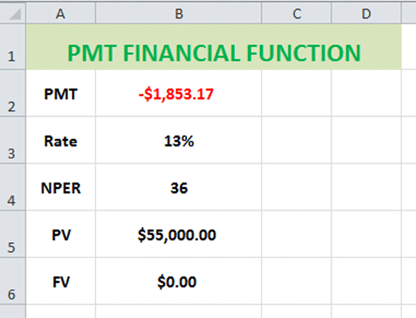
PMT = monthly instalment (if this is an investment and you are receiving the payment, it will be a positive number).
Rate = interest rate (the interest rate divided by the number of months in a year to calculate monthly interest, for example, 13%/12).
NPER = the number of payments/instalments to be made. In the screenshot above, there are 36 instalments
(3 years multiplied by 12 months).
PV = this is the total amount of the loan or the present value. It can be positive, if you need to repay it, or negative, if you are providing a loan to someone else.
FV = this argument is not always necessary. It is the future value of the loan after the last payment has been made.
The best method of learning how to use the PMT and other financial functions is to recreate the examples given in this tutorial and to follow each step by completing it in Excel.
Let’s begin by creating a PMT calculation.
* Calculate Monthly Payments Excel ~ PMT Excel
Imagine you wish to buy your fiancé a beautiful diamond ring or you want to know whether you can actually afford to buy the latest Apple Watch or iPhone. You may even have a much larger purchase in mind, for example an apartment or your dream car.
The PMT function allows you to see how close your dreams are to the reality of what you can afford. It allows you to play with different variables, for example, paying a loan off over 10 years instead of three, to see how this affects the monthly payment amount.
For our scenario, let’s imagine you wish to purchase a car that costs $125,000. When calculating your monthly budget, you realize you can afford to pay a maximum of $2,800 per month to finance a car. The Bank indicates the interest rate will be 18% annually if you take the loan over 5 years.
Start by creating a new worksheet and inserting the fields as per the screenshot below:
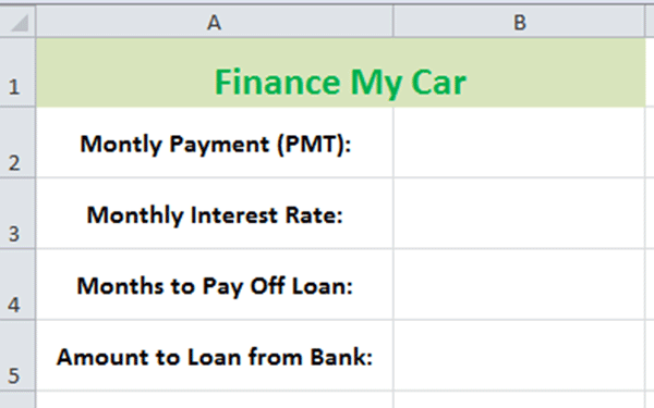
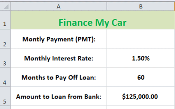
1. First let’s calculate the monthly interest rate. The bank has indicated an annual interest rate of 18% and therefore we can calculate the monthly interest rate by dividing it by the 12 months in a year (18%/12). Enter 1.50% in the Monthly Interest Rate cell (B3). Remember to apply the Percentage format to this cell to ensure it displays correctly.
2. Next, let’s calculate the number of months you are paying the loan off over. The bank is giving the loan over a period of 5 years. To calculate the number of months, you multiply the years by 12 (5*12), which equal 60 for the number of months. Enter 60 into the cell next to: Months to Pay Off Loan (B4). Remember to apply the Number format to this cell.
3. The amount you wish to loan from the bank is $125,000. Enter this amount into the cell next to the Amount to Loan from Bank (B5). Remember to apply the Currency format to this cell.
Your worksheet should resemble the screenshot below:
4. The final piece of the puzzle is the PMT function. You need to insert this in the B column next to the Monthly Payment (PMT) cell (B2).
Type: =PMT(
The formula will suggest the following syntax in the screen tip:
=PMT(rate, nper, pv, [fv], [type])
(FV (Future Value) and Type are both optional and we will not be using them in our example.)
5. After typing: =PMT( , click in the cell containing the rate: 1.50% (B3), followed by a comma.
6. Next, select the number of payments: the cell containing 60 (B4), followed by a comma.
7. Finally, select the loan value (PV), which is $125,000 (B5) in our example. Close the brackets after selecting this cell and press the Enter key.
The completed formula should look like this:
=PMT(B3,B4,B5)
The result for the monthly payment should have calculated as: -$3,174.18.
Below is a screenshot with the completed formula in the Formula Bar:
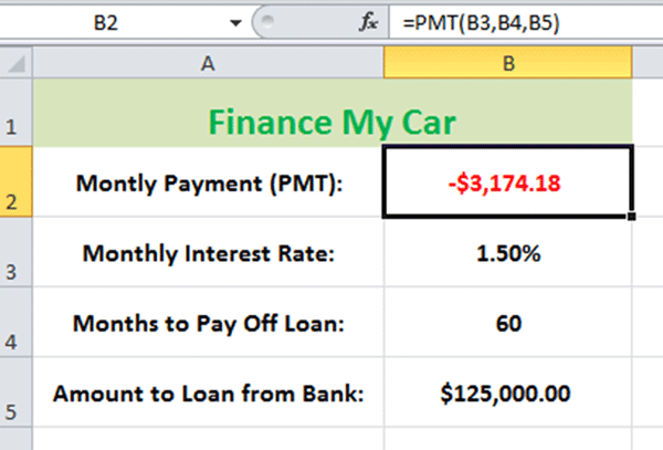
It is clear that this loan is therefore not affordable as at the beginning of this scenario we indicated we could afford to pay only $2,800 per month.
You can now play around with the values in the Rate, NPER and PV cells to calculate under which conditions you could afford the loan.
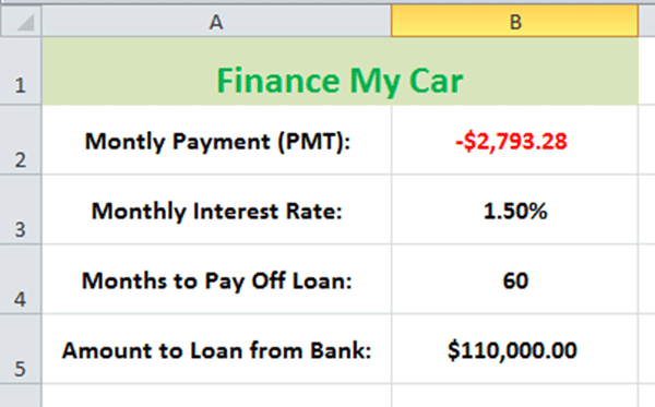
For example, changing the number of months over which to pay it off or buying a slightly less expensive car of around $110,000, will make the PMT value fall below the $2,800 affordability mark:
Have fun experimenting with changing variables and seeing how close you can come to your own dream-purchase!
* Calculate Interest Rate in Excel ~ Rate Excel
There are many instances where the interest rate is either not available or you wish to calculate it based on variables such as the total loan amount and monthly payments.
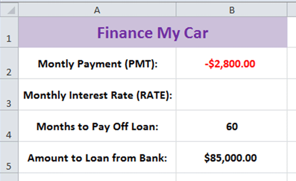
To calculate only the rate, make a duplicate of the worksheet created in the tutorial above and replace the formula in cell B2 (next to PMT) with a negative amount (-2800 in our example below). Also delete the interest rate contained in the Rate cell (B3).
Your worksheet should resemble the screenshot below:
To calculate the interest RATE:
1. In cell B3 (next to Monthly Interest Rate), type the following formula:
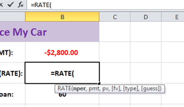
=RATE(
Excel will provide the formula syntax in a screen tip (see screenshot below):
2. Select cell B4 which contains the number of payments (NPER), followed by a comma.
3. Next select cell B2 which contains the monthly payment (PMT) value, followed by a comma.
4. Finally, select cell B5 which contains the total loan amount (PV), followed by a comma. Close the brackets and press the Enter key to accept the formula.
The completed formula and result for this example should resemble the screenshot below:
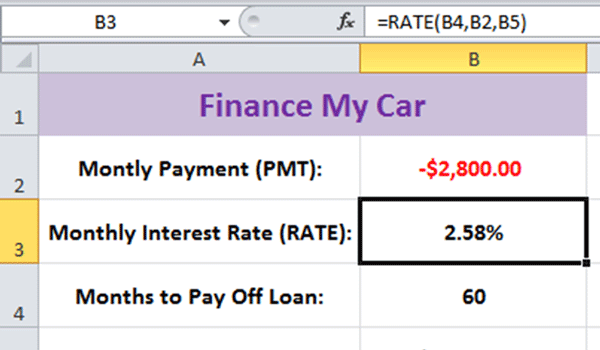
The monthly interest rate is calculated as 2.58% based on the other variables you completed.
* Calculate Number of Payments ~ NPER Excel
No one likes to owe money, but at times it is necessary in order to make a high value purchase. Most people wish to be able to pay the loan off as quickly as possible, but this is not always possible, especially when the loan amount is high.
If you have the monthly instalment (PMT), monthly interest rate (RATE) and total amount of the loan (PV) variables available, you can calculate the number of months needed to pay off a loan.
Save a copy of the worksheet you created for the above tutorial and replace the values as demonstrated in the screenshot below:
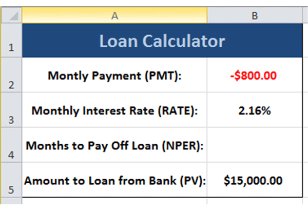
Based on the variables in the screenshot example above, to calculate the number of months this loan will take to pay off over, do the following:
1. In cell B4 (next to NPER), type the formula:
=NPER(
Excel will provide the syntax for this formula in a screen tip, as demonstrated in the screenshot below:
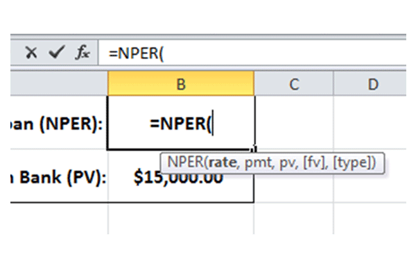
2. Select the cell containing the rate (B3) and insert a comma.
3. Select the cell containing the PMT value (B2) and insert a comma.
4. Finally, select the cell containing the PV value (B5). Close the brackets and press the Enter key to finalize the formula.
If you followed the example above, your NPER value should be 24 months.
See screenshot below for completed formula in the Formula Bar:

Experiment with changing the variables for RATE, PMT and PV to calculate how many months the loan can be paid off over.
* Calculate Amount You Can Afford to Loan ~ PV Excel
If you are the sensible type, you probably want to calculate how much money you can safely afford to lend before committing yourself to a purchase. You base this on the amount you can afford to pay monthly, relevant interest rate and over how many months you want to be paying it off.
For example, after working out her budget, Sarah calculates she can put $700 per month towards a car payment. Ideally, she would not like to pay off a car for more than three years (36 months) and her bank’s current interest rate is a whopping 23% per annum (1.92% per month).
To calculate this, save the worksheet you created in the previous tutorial and replace the values in each cell as indicated in the screenshot below:

To calculate the amount Sarah can afford to lend from the bank based on the variables above:
1. In cell B5 (PV) type the formula:
=PV(
Excel will suggest the syntax for this formula as demonstrated in the screen tip in the screenshot below:

2. Select the RATE cell (B3) followed by a comma.
3. Next, select the NPER cell (B4) followed by a comma.
4. Finally, select the PMT cell (B2). Close the brackets and press the Enter key to accept the formula.
If you followed the values in the example above, your PV value should be: $18,073.58.
This means, based on the variables that were entered for the amount Sarah can afford monthly, the number of months she wish to pay off the loan over and her bank’s interest rate, she can afford to buy a car of around $18,000.
Go back to the worksheets you created for calculating the PMT, NPER, RATE and PV, review each formula and experiment with different variables. Next, impress your friends by showing them your financial savvy calculations for everything from paying off a student loan to buying a house!
Woohoo! Now that you have done the tutorial:
Test your Excel skills with the corresponding FREE Online Multiple Choice
Financial Functions in Excel Test
TRY THE NEXT TUTORIAL: Formatting Spreadsheets in Excel ~ Basic Worksheet Formatting Tutorial
TRY THE NEXT TEST: Formatting Spreadsheets in Excel ~ Basic Worksheet Formatting Test


