www.TestsTestsTests.com
Aligning Cell Content in Excel Tutorial
Excel 2016 Tutorial
Data Entry and Formatting in Excel
Free Online Microsoft Excel Tutorials – 2016
* Horizontal, Vertical and Diagonal Cell Alignment in Excel 2016
* Horizontal Cell Alignment
* Vertical Cell Alignment
* Diagonal Cell Alignment
* Wrap Text in a Cell
* Merge and Center in Excel – Cell Content
* Indent Cell Content in Excel 2016
|
Use the Alignment Group tools in Excel to merge headings across columns and rows, change the position of text within a cell and set horizontal and vertical alignment of data to improve readability. |
 |
* Horizontal, Vertical and Diagonal Cell Alignment in Excel 2016
Did you know you can set the position of text and numbers within a cell? Excel 2016 for Office 365 contains all the cell alignment functions that have been with MS Excel for more than a decade and makes it easier than ever to set alignment for cell content.
You can align text vertically, horizontally and diagonally. There are also rotation options where you can rotate the cell content by a set degree. Let’s look at how you can do this.
* Horizontal Cell Alignment
Firstly, let’s see what steps you need to take to set Horizontal Alignment:
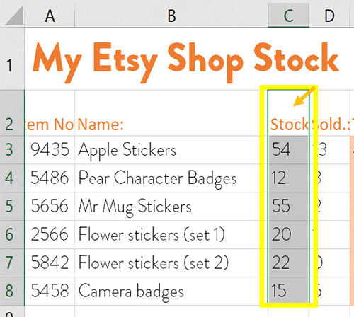
1. Select the cell(s), rows or columns you want to apply Horizontal Alignment to (see selection outlined in yellow in the screenshot below):
2. Under the Home tab on the Ribbon, find the Alignment group. Select from left, right or center cell alignment options (outlined in yellow in the screenshot below):

3. If you look closely at the icons you will notice that the way the lines on the buttons display indicate the type of alignment that pressing the button provides: left, center or right. Click a button for the alignment you wish to apply.
TIP: Experiment with the three Horizontal Alignment types to see how it will look when applied in your worksheet.
* Vertical Cell Alignment
Next, let’s see what steps you need to take to set Vertical Alignment.
1. Select the cell(s), rows or columns you want to apply Vertical Alignment to.
2. Under the Home tab on the Ribbon, in the Alignment group, select from top, middle and bottom cell alignment options (outlined in yellow in the screenshot below):

3. If you look closely at the icons (outlined in yellow in the screenshot above) you will notice that the way the lines on the button display indicate the type of alignment pressing that button provides: top, center and bottom of cell. Click to apply one of the alignment types.
TIP: Experiment with the three alignment Vertical Alignment types to see how it will look when applied in your worksheet.
* Diagonal Cell Alignment
The third alignment option is Diagonal Alignment, which allows you display cell contents diagonally at any angle. This option is useful when you have limited space in a worksheet as you may be able to fit more content on a page with diagonally populated cells. It can also be used to make a worksheet look professional and aesthetically pleasing.
Let’s look at the steps you need to follow to set Diagonal Alignment:
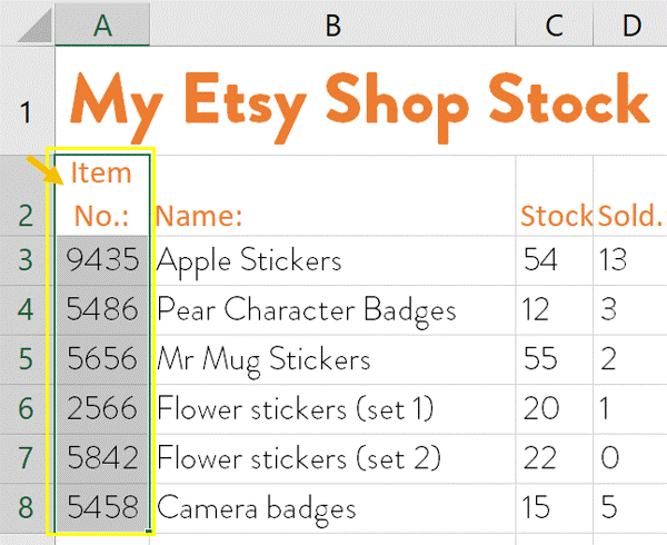
1. Select the cell(s), rows or columns you want to apply the Diagonal Alignment to. In the screenshot below, cells A2 to A8 is selected (see outlined in yellow):
2. Under the Home tab in the Alignment group, look for the Orientation button (outlined in yellow in the screenshot below)

3. Click the Orientation button and select from the following options: Angle Counterclockwise, Angle Clockwise, Vertical Text, Rotate Text Up and Rotate Text Down. If you look closely at the icon for each of these option – the direction of the arrow and text indicates how the alignment will look when applied.
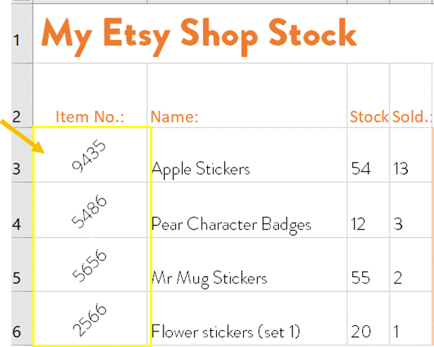
For our example, we selected Angle Counterclockwise – see screenshot below for how this alignment looks when applied:
To remove Diagonal alignment: Go to the Home tab and in the Alignment Group, click on the dialog box launcher (labelled A) to open the Alignment dialog box (labelled B) – as outlined in the screenshot below:
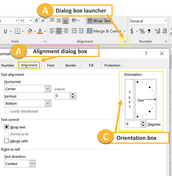
In the Orientation box (labelled C in the screenshot above) change the Degrees option to 0 and press OK. This will remove the Diagonal Alignment formatting from your selected cell(s), rows or columns.
The Alignment dialog box also offers more detailed options for changing horizontal and vertical alignment. Go ahead and experiment with different alignment settings in your Excel worksheet.
* Wrap Text in a Cell
This is probably one of the issues people struggle with most when they first start working in Excel. When you type text into a cell it appears to run over multiple cells or can even appear to be hidden behind other cell content.
In the screenshot below, Cells A10, B10 and C10 contain text that is difficult to read and clearly has some text missing:
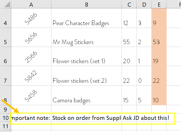
There is one button that can quickly fix this issue for you and that is the Wrap Text option.
To apply this option:
1. Select the cell or cells you wish to apply Wrap Text to – in our example this will be A10, B10 and C10.
2. Under the Home tab in the Alignment group find the Wrap Text button (outlined in yellow in the screenshot below):
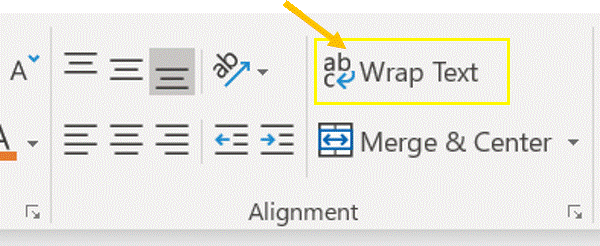
3. Click to apply this option and the row will enlarge to accommodate and display all of the cell content.
TIP: Drag the column divider to increase the width of a cell to make the content fit better into your worksheet layout.
* Merge and Center in Excel – Cell Content
After applying the Wrap Text option, you may find that the cell content is now confined to one cell where you may have wanted it to cross over multiple cells, the width of your worksheet. This is often an issue with headings where you may want it to be top center of all the worksheet columns.
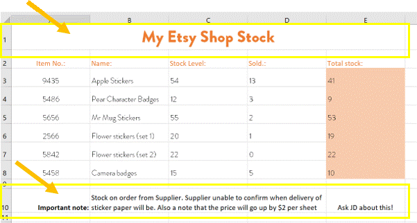
In the example below the heading of the worksheet – My Etsy Shop Stock – is currently positioned on the left of the worksheet and despite applying the Center Alignment (discussed at the beginning of this tutorial), the heading is still on the left-hand side of the worksheet. This is where the Merge and Center function comes in useful.
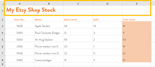
To Merge and Center cell content:
1. Select the cell you want to merge AS WELL as the cells you want to merge it across. In the example screenshot above, we would select cells A1 to E1.
2. Under the Home tab on the Ribbon, in the Alignment group, click on the Merge and Center button (outlined in yellow in the screenshot below:
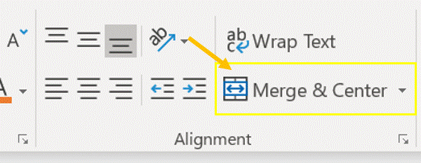
With this option applied, our heading has moved to the top center across all the cells selected. We have also applied Merge and Center, as well as alignment options, to the contents of Row 10 in the worksheet. Compare the screenshot below to the ones earlier in this tutorial to see what a difference the Merge and Center function makes.
* Indent Cell Content in Excel 2016
Indenting text or numbers in a cell can help make your worksheet look neater and make contents easier to read and understand.
To apply the Indents function to cell(s), rows or columns in a worksheet:
1. Select the cells you want to format.
2. Under the Home tab, in the Alignment group, click on the Increase Indent button (A) to indent the cell contents. Use the Decrease Indent button (B) to reduce the indent applied.
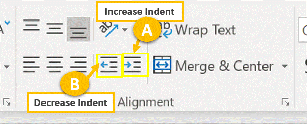
TIP: You can press the Increase Index button multiple times to increase the indent within a cell or multiple cells.
Woohoo! Now that you have done the tutorial:
Test your Excel skills with the corresponding FREE Online Multiple Choice
Aligning Cell Content in Excel 2016 Test – Data Entry and Formatting
TRY THE NEXT TUTORIAL:
Customizing Number & Text Formats in Excel Tutorial
TRY THE NEXT TEST:
Customizing Number & Text Formats in Excel Test


