
www.TestsTestsTests.com

Add Text in Excel – Add Numbers in Excel
Excel Spreadsheet & Worksheet Tutorial
Excel 2016 Tutorial
Data Entry and Formatting in Excel
Free Online Microsoft Excel Tutorial
* Add Text in Excel – Add Numbers in Excel 2016
* How to align Excel cell content
* Resizing rows and columns to fit cell contents
in Excel 2016
* Fitting contents to column width
in Excel 2016
* How to add paragraphs to cells
* How to edit and delete cell contents
|
Adding text or numerical values to a worksheet requires the ability to insert, edit, fit and delete cell contents. Master the Excel grid of cells, rows and columns by adding headings, paragraphs, row or column headings and capturing values. |
 |
* Add Text in Excel – Add Numbers in Excel 2016
When you use Microsoft Excel for the first few times and attempt to insert data such as text or numbers, you may find the Excel screen puzzling. Different to normal text editors, the Excel screen is made up of a grid, not a blank page, and data is organized into rows and columns comprising cells. It is important to get a good grasp on how the Microsoft Excel screen is organized. For a refresher course on this, see our The Different Parts of the Excel 2016 Screen Tutorial and Test.
Excel’s grid helps you to organize data with column or row headings. A good place to start is to look at the data you wish to add to an Excel worksheet and, if the data doesn’t already have, create column or row labels for each data type. For example, you may want to add all the names, ages and grades of students in your class to a worksheet.
So how do we do this in Excel?
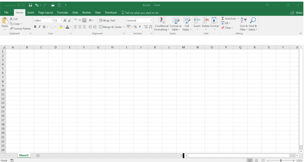
1. Open your copy of Microsoft Excel 2016 where a blank worksheet will open by default resembling the screenshot below:
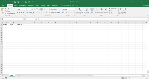
2. Click once in the first cell (cell A1) and then type the word: NAME
3. Press the Tab key on your keyboard to move to the next cell (B1) and type the word: AGE
4. Press the Tab key again and type the word: GRADE into cell (C1)
Good job! Your sheet should now look something like this:
The next step is to start filling out the data for each of these column headings, i.e. NAME, AGE and GRADE.
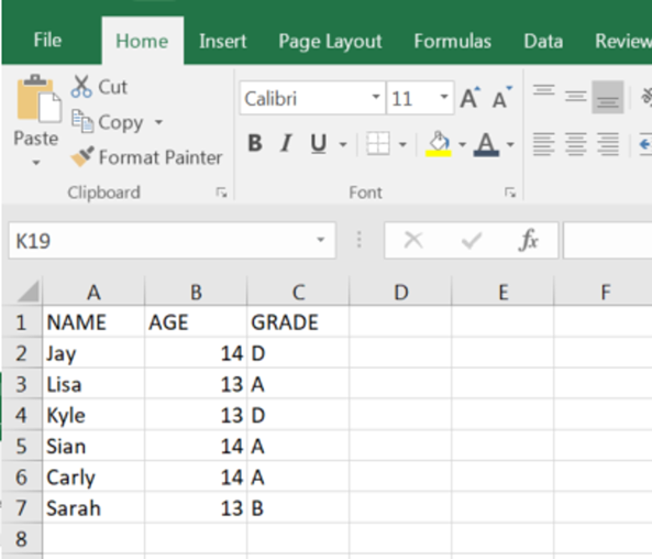
1. Click in the cell below NAME (cell A2) and type a name (any name – be creative!). Press the Tab key to move to the next cells, in the columns labelled AGEand GRADE, respectively, and add data.
2. After inserting a value under the GRADE heading, press the Enter key on your keyboard to move to the next row (Row 3) and add a second line of data.
How did you do? Were you able to add data to your worksheet so that it looks like the example worksheet below?
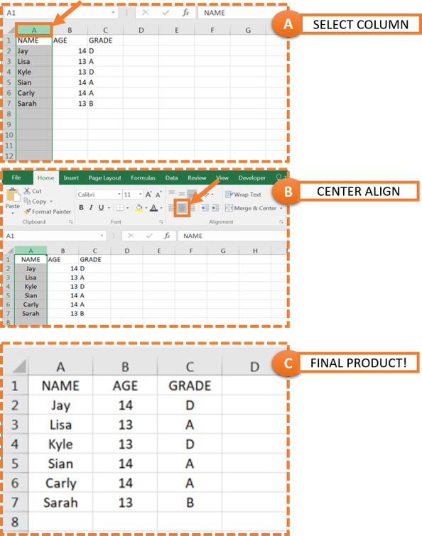
* How to align Excel cell content
Looking at the worksheet we created in the screenshot above, you may notice that some of the content is positioned to the left and some to the right of the column heading, resulting in a misaligned look. To align text in a cell we can use Left, Center and Right alignment.
To align cell contents:
1. Select the column you wish to change alignment for by clicking on the column label. The column label is represented by a letter of the alphabet, so, for example if you want to select the NAME column in our example above, you will click on the A column label.
2. Next, with the column still selected, click on the Home tab on the Ribbon and in the Alignment group, click on the Center button.
3. Now repeat step 1 and 2 above for the other two columns on your sheet (AGE and GRADE).
Aligning data in a worksheet is as easy as A, B, C! See our screenshot below for a quick visual summary of the three steps:
Other alignment options include Right, Left, Top, Middle, Bottom and indents. Go ahead and experiment with these options too!
* Resizing rows and columns to fit cell contents in Excel 2016
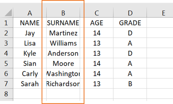
Rows and columns can be resized to fit the contents of a cell or be sized to make your worksheet look neat. When you add text or numbers to a cell, part of the text may be obscured. Have a look at column B (outlined in orange in the screenshot below. You will note part of the surnames in column B are obscured (specifically Washington and Richardson):
We can resize column B to ensure the content is visible by following any of the options set out below:
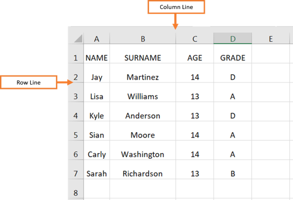
1. Drag the column lines to enlarge the cell width (see screenshot below). Click on the column line to the right of the column labelled B, hold down your mouse button and drag it to the right to enlarge the column.
OR
2. Double-click the column line on either side of the column labelled B to automatically resize the column to fit the contents.
TIP: Resize selected columns at the same time to ensure the columns are all equally distributed by selecting all the columns you wish to resize and then dragging the line to the right or left of the column to resize.
Rows can be resized in the same way as columns:
1. Drag the lines of an individual row downwards or upwards to increase or decrease the row height.
OR
2. Double click on the line above or below the row label to automatically resize the row to fit its contents.
TIP: Resize selected rows at the same time to ensure the rows are all equally distributed by selecting all the rows you wish to resize and then dragging the line above or below the row label to resize.
Practice resizing individual’s rows and columns and selected groups of rows and columns until you’ve mastered it!
* Fitting contents to column width in Excel 2016
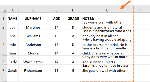
Resizing a column to fit its contents isn’t always the solution you need, especially if the cell contents is several lines long and you need for it to fit into a specified space for printing or aesthetic reasons.
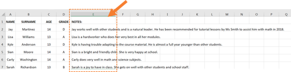
Consider the screenshot below: the contents of column E is considerably longer than the current column width. This can be rectified by resizing the column width (as discussed in the previous section) or the text can be wrapped within a column width to ensure a better fit. This is especially suitable for cells containing long lines of text.
To wrap (or fit) a paragraph within a specified column width:
1. Select the cell(s) or entire column containing the text you wish to fit into the column width.
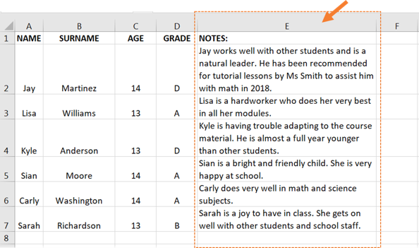
2. Under the Home tab on the Ribbon in the Alignment group, click on Wrap Text.
This will wrap the text lines into the column width:
The next step is to resize the row height to fit the contents. You can also adjust the column width, either increasing or decreasing the width. To resize the row height, select the rows and drag the row line on any of the rows downwards to increase the row height.
TIP: Apply the Wrap Text function to blank cells you may later wish to fit into the designated space. This will make adding data to cells at a later stage, easier.
* How to add paragraphs to cells
Breaking up text within the same cell into paragraphs is quite a neat trick in Excel, a shortcut key combination that is worth writing on a post-it note and sticking it on your computer screen.
If you want to add another paragraph to text within the same cell in Excel:
1. If the cell you wish to add the paragraph to isn’t currently selected, double-click the cell to select and edit the cell contents.
2. Move the cursor to the end of the text to the spot where you wish to insert or break the text up into another paragraph.
3. Hold down the Alt key on your keyboard and press the Enter key to create a new paragraph (see screenshot below for the end result).

You can add as many paragraphs within the same cell as you wish!
* How to edit and delete cell contents
Now that you’ve mastered adding text and numbers, creating row and column labels, resizing rows and columns to accommodate cell contents, and wrapping contents to ensure it fits within the column width, let’s look at how to edit and delete cell contents.
1. To delete the contents of a cell, select the cell by clicking on it once. Press the Delete button on your keyboard.
2. To delete the contents of a row or column, select the row or column by clicking on their label (e.g. column A, Row 1, etc) and press the Delete button on your keyboard.
For more advanced Delete options:
1. Select the cell, row or column you wish to delete; and
2. Under the Home tab on the Ribbon, in the Cells group, click on the dropdown arrow below the Delete button:
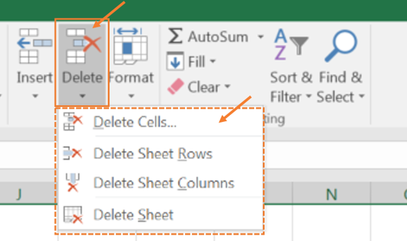
You can select to Delete Cells, Delete Rows, Delete Columns and Delete Sheet quickly using these options.
Woohoo! Now that you have done the tutorial:
Test your Excel skills with the corresponding FREE Online Multiple Choice
Adding Text and Numbers to a Spreadsheet / Worksheet – 2016 Excel Basics Test
TRY THE NEXT TUTORIAL:
Formatting Text In Excel ~ Formatting Numbers Excel Tutorial
TRY THE NEXT TEST:
Formatting Text In Excel ~ Formatting Numbers Excel Test