www.TestsTestsTests.com
Conditional Formatting Excel Tutorial
Excel 2010 Training –
Working with Data
Free Online Microsoft Excel Tutorial
* What is Conditional Formatting?
*
Highlight Cell Rules
* Top and Bottom Rules
* Manage Rules
* Remove Rules
Conditional Formatting lets you highlight data. You can apply different formatting to a cell or cells that meet your specific conditions i.e. all cells over $5000 or the top 10 items or all of the cells within a date range. This can help you focus on what’s really important.
Test your Excel skills with the corresponding FREE Online Multiple Choice
Conditional Formatting Excel Test
* What is Conditional Formatting?
Conditional formatting is arguably one of Excel’s most useful and fun features. It allows you to quickly create a visual analysis of a worksheet by applying formatting to specified cells based on their contents. You can, for example, decide that all cells containing the word YES must be formatted with green font and all cells containing the word NO, should be formatted in red font.
You can create conditional formatting rules for just about any condition. If you apply conditional formatting to an entire worksheet, the rule will continue to be applied to data that you add or change on the worksheet. Conditional formatting is a great timesaving tool that ensures consistency and accuracy in formatting data using the same formatting rules.
Study the screenshot below. A conditional formatting rule that displays amounts lower than $15,000 in red font and amounts higher than $15,000 in blue font, has been applied to the Salary column. A conditional format that highlights cells that contain the word YES in green and the word NO in red, has been applied to the Pass column:
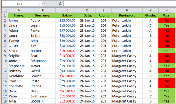
Conditional formatting is a replacement for manually finding and formatting individual cells or groups of cells and also automatically adapts to any changes made to the contents of a cell. For example, if a NO in the Pass column (see screenshot above) was changed to a YES, the cell will automatically be reformatted to green shading.
There are literally thousands of variations of conditions and formatting types that can be set and it is worth having a look through the available options.
To experiment with conditional formatting options:
1. In an open worksheet, click on the Home tab on the Ribbon.
2. In the Styles group, click on the Conditional Formatting button. This will open a menu list with available categories of conditional formatting (see menu circled in yellow in screenshot below). Each category has several subcategories that you can explore individually.
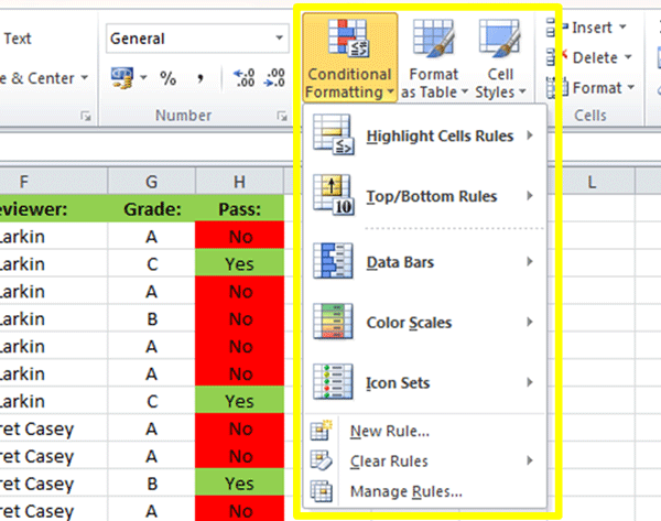
Depending on the type of data and how you wish to format it, you will find an option in the conditional formatting list.
Next we look in more detail at how to apply conditional formatting.
* Highlight Cell Rules
The Highlight Cell Rules option allows you to apply conditional formatting based on conditions such as:
- * Greater than…
- * Less than…
- * Between…
- * Equal to…
- * Text that contains…
- * A date occurring…
- * Duplicate values…
Depending on the type of data you wish to analyze you can pick one of these options or click on More Rules to customize a condition.
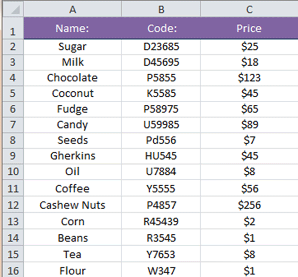
For example, say we have a worksheet containing a price list of items and we want to ensure that whenever a price higher than a specific amount is entered, the cell changes color automatically (see Price column in the screenshot below):
To apply a Highlight Cell rule:
1. Select the data you wish to apply the formatting to. In our example in the screenshot above it will be the Price column.
2. Select the Home tab on the Ribbon and then in the Styles group, click on the Conditional Formatting button.
3. Select Highlights Cells Rules from the menu list and then select Greater Than. This will open the Greater Than dialogue box.
4. In the Format cells that are GREATER THAN box, type the value that forms the basis for the rule, i.e. all cells that contain a value that is larger than the one you entered will have the conditional formatting applied to it automatically. In our example in the screenshot above, we wish that all cells that contain values that are greater than $50 be formatted.
5. After entering the base value, click on the dropdown arrow next to the formatting list (circled in yellow in the screenshot below):
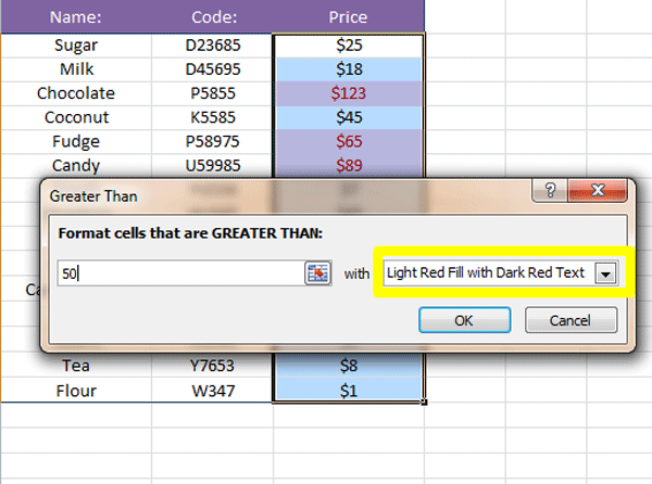
6. From the dropdown list, either select one of the preformatted cell options, for example Light Red Fill with Dark Red Text, Green Fill with Dark Green Text, etc., or select the Custom Format option.
7. The Custom Format option will launch the Format Cells dialogue box. From here you can apply any formatting combinations that comprise number formatting, font, cell borders and cell fills. Make a selection for how you wish the cells to be formatted and press OK.
The cells containing values that match the conditional formatting rule you applied, will be automatically formatted. If you change the values in the cell range to which the conditional formatting is applied, the formatting will automatically be applied to cells that meet the requirements.
* Top and Bottom Rules
Have you ever looked at a list of numbers in Excel and wished you could quickly get a visual analysis of the top performers, or the bottom performers or those above or below average? Conditional formatting allows you to quickly analyze a sheet without complex formulas or data analysis skills. Applying conditional formatting also changes the formatting from static to dynamic in that it will change as data entered on the worksheet changes, ensuring you can get a quick visual analysis of the data.
To apply a Top and Bottom Rule:
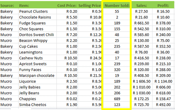
1. Select the data series you wish to apply the conditional formatting to. In the screenshot below, we wish to analyze the top performers by the Number Sold column:
2. Select the Home tab on the Ribbon and then in the Styles group, click on the Conditional Formatting button.
3. From the Conditional Formatting menu list, select the Top and Bottom Rules option.
4. From the submenu list for Top and Bottom Rules there are a number of useful options which are circled in yellow in the screenshot below:
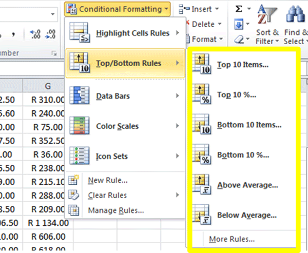
5. To highlight the top selling items by Number Sold, we can select the Top 10 Items rule.
6. In the Top 10 Items dialogue box, enter the number for the top performers in the Format cells that rank in the TOP box. In our example, we want to know the top 5 selling items by number.
7. Next, we select the formatting we wish to apply to the top five performers. Either select one of the pre-set formats in the list or click on Custom Format to set number format, font, cell borders and cell shading.
This is a great tool to quickly analyze a list where you need to see top or bottom performers or above or below average numbers. As mentioned in the previous lesson, conditional formatting is dynamic and the formatting will change as the values change. For example, if the data on the worksheet changes so that the top performers from last week are no longer the top performer based on new values entered, the formatting will automatically adjust to reflect the new top items.
* Manage Rules
Over a period of time, you may find that you have applied so many different conditional formatting rules to a worksheet that the rules are no longer working as expected. This could happen, for example, when one rule literally overrules another rule if they are applied to the same selection of cells.
The Conditional Formatting Rules Manager allows you to not only view all the rules applied to the worksheet or selected cells, you can also use it to delete rules, edit rules and create new rules. You can even use it to manage the order in which rules are executed and change the cell ranges they apply to.
To use the Conditional Formatting Rules Manager:
1. Select the entire worksheet or cell range that contains the conditional formatting rules you want to manage.
2. Select the Home tab on the Ribbon and in the Styles group, click on the Conditional Formatting button.
3. Select Manage Rules from the Conditional Formatting menu list. This will launch the Conditional Formatting Rules Manager dialogue box (see screenshot below):
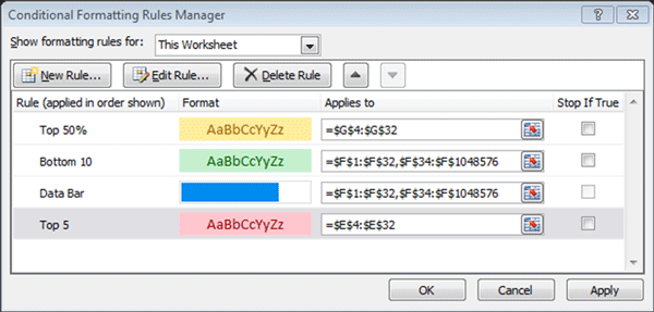
4. You can view all the rules that are applied to the current selection, the current worksheet or any other worksheets in your workbook, by selecting the relevant option from the Show formatting rules for: dropdown list at the top left-hand corner of the dialogue box.
5 To edit a specific rule, select the rule by clicking on it in the box and then click on Edit Rule. This will take you to the Edit Formatting Rule dialogue box (see screenshot below):
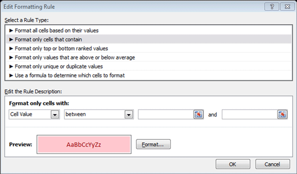
6. In the Edit Formatting Rule dialogue box, you can change the rule type, edit the rule function and change the format that is applied to cells that meet the rule conditions.
7. Press OK to accept any edits you make to a rule.
The Conditional Formatting Rules Manager is an essential tool when working with conditional formatting. It is also useful for ascertaining whether a worksheet has any conditional formatting rules applied to it, especially if the worksheet was created by someone else.
* Remove Rules
Conditional formatting rules are often used once off just to analyze a worksheet and need to be removed after a visual analysis has been concluded. At other times due to changes in data type or needs, they may have been replaced without the old rule being deleted. The most common reason for needing to remove conditional formatting rules, however, is due to duplicate or incomplete rules that were created.
To remove conditional formatting rules, it is important to first establish what rule it is you wish to remove and from what part of the data.
1. Select either the entire worksheet by pressing Ctr+A or select the cell range containing the rules you want to remove.
2. Ensure the Home tab on the Ribbon is selected and the click on the Conditional Formatting button in the Styles group.
3. To delete all rules that have been applied to the worksheet or selected cell range, click on Clear All in the Conditional Formatting menu list and select either Clear Rules from Selected Cells or Clear Rules from Entire Sheet.
4. To delete specific rules only, click on the Conditional Formatting button in the Styles group and select Manage Rules from the menu list. In the Manage Rules dialogue box, select the rule you wish to delete and click on the Delete Rule button.
If you delete a rule in error and wish to reinstate it, use the Undo button or Ctrl+Z to reverse the delete or remove action.
Now you have done the tutorial…
Test your Excel skills with the corresponding FREE Online Multiple Choice
Conditional Formatting Excel Test
* TRY THE NEXT TEST: Using Data Validation Tools in Excel


