www.TestsTestsTests.com
Formatting Numbers Excel Tutorial
Free Online Microsoft Excel 2010 Tutorial
Excel Formulas and Functions
* General Formatting in Excel
*
How to change Decimal Places in Excel
*
How to change Currency in Excel
*
Negative Numbers in Excel
*
Formatting Dates in Excel – change format of date in Excel
*
Formatting Fractions in Excel
You want numbers to appear correctly. This is done by formatting numbers for currency, percentage, dates, and fractions including decimal places and negative numbers.
Test your Excel skills with the corresponding FREE Online Multiple Choice
Formatting Numbers Excel Test
* General Formatting in Excel
A distraught friend once came to me with a spreadsheet which needed to contain multiple phone numbers, but Excel automatically kept turning the phone numbers into exponential numbers or hash symbols. She was just about pulling her hair out as all she wanted was the numbers to display as phone numbers! She was rather shocked to find it was just a formatting setting that is one or two clicks away.
Telephone numbers are not the only instance when Excel seemingly misbehaves. Entering dates, percentages or currency into a spreadsheet can all yield unexpected results.
It is therefore essential to understand how number formats work and where to change them in order to work successfully (and should we say peacefully) with Excel.
Should you wish the numbers you enter into Excel to be formatted and understood by Excel as numbers, do the following:
1. Select the cells, columns or rows you wish to format as numbers.
2. Under the Home tab on the Ribbon, go to the Number group and click the dropdown arrow next to the selection box (circled in yellow in the screenshot below):
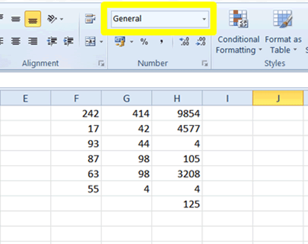
3. From the dropdown list select General or Number.
Your cells will now be formatted as numbers and Excel will treat them as numerical values.
Oftentimes if a formula is not working as expected it may be that the formatting of the cell contents is to blame. Numbers may have been formatted, for example, as text, which will cause values entered into a cell to display as numbers, but the format of the cell is text. Excel will treat numbers formatted as text as if they were words and not numerical values which will cause formulas not to work properly.
Study the screenshot below:
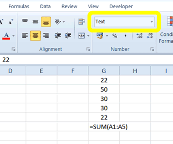
You may note the number format of the cells in column G is Text (circled in yellow above) even though numbers are displaying in the cells and formula bar. The result is a formula that displays as text instead of calculating the values.
To correct the problem in the above example we need to format numerical values as numbers:
1. Select the cells, rows or columns to format as numbers. In the example above that would be cells G1:G6.
2. Click on the Home tab on the Ribbon.
3. In the Number group click on the dropdown arrow next to Text in the format selection box and choose Number from the list of available formats by simply clicking on it:
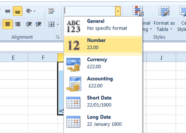
Numerical values will now be formatted as numbers instead of text. If you used formulas (like we did in our example) you will need to delete and re-insert the formula. It may seem confusing that although the content of the cells in the above example displayed as numbers in both the cells and the Formula Bar, that because of their formatting Excel treated them as if they contained text. A simple way of understanding this is to see number formatting as the tinted lens Excel sees a cell through. We need to change the lens to the correct formatting for Excel to treat the content correctly.
* Decimal Numbers – How to change Decimal Places in Excel
When working with numbers, decimals play an integral part in everything from separating cents from dollars in monetary values to indicating minute fractions of larger numbers such as the n-th digit of Pi.
Decimals date back to the 1st century AD when Chinese mathematicians invented it for calculating fractions. From there it spread to the Middle East, then Europe and now a Microsoft Excel spreadsheet near you with the click of a button!
To increase or decrease decimal places visible in cells that contain numbers:
1. Select the cells, rows or columns containing the values of which you wish to increase or decrease decimal places for.
2. In the Number group under the Home tab on the Ribbon, click on the Increase Decimal or Decrease Decimal buttons (circled in yellow in the screenshot below) for however many decimals you wish to increase or decrease on the selected cells.
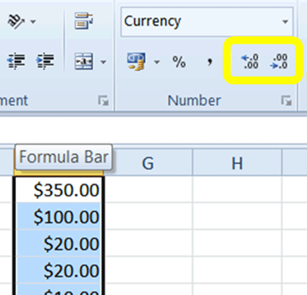
Note: Excel will automatically round up decimals to the nearest whole number if you use the Decrease Decimal button to decrease decimals until only the integer (a whole number) is on display
* How to change Currency in Excel
One of the main uses of spreadsheets is for financial records and calculations. It therefore stands to reason that currency plays an important part in the formatting of spreadsheets. Excel comes pre-packed with just about every currency symbol in existence. Using the currency formatting to insert a currency symbol does not only save you time from having to insert the symbols manually, it also ensures numbers are treated as currency and calculated correctly in formulas without typed symbols getting in the way.
To format cells as currency and include a currency symbol:
1. Select the cells, rows or columns you wish to format with a specific currency symbol.
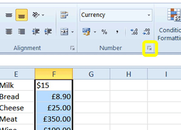
2. Under the Home tab on the Ribbon in the Number group, click on the dialogue box launcher (circled in yellow in the screenshot below). This will launch the Format Cells dialogue box.
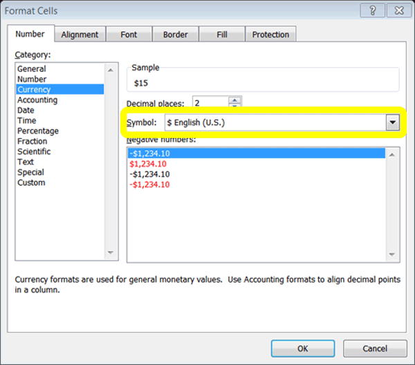
3. In the Format Cells dialogue box click on the Number tab and select Currency from the Category group.
4. Select the correct symbol for the currency format you require from the symbol dropdown list (circled in yellow in the screenshot below):
5. Press OK to accept the currency format.
Your cell selection will now automatically be formatted with the currency symbol you selected.
Note: If the cells you are formatting contain a manually inserted currency symbol, you will need to delete these before the currency formatting will take effect.
TIP: You can apply number formatting, such as currency, to blank cells, rows and columns so that any numbers inserted there will automatically be formatted with the correct number format.
* Negative Numbers in Excel
Negative numbers are essential when working with spreadsheets indicating, for example, the debits or outstanding amounts on an account.
Specific formatting can be applied to negative numbers to ensure they are easy to see. For example, you could indicate that any numbers in a column that is inserted and prefixed by a minus symbol, needs to be formatted in red font. Additionally, by applying formatting to cells containing formulas to format negative numbers a certain way, may make it easy for people interpreting the spreadsheet to clearly see where there is a negative or positive value.
To set number formatting for negative numbers:
1. Select the cells, rows or columns to apply the number formatting to.
2. Launch the Format Cells dialogue box and ensure the Number tab is selected.
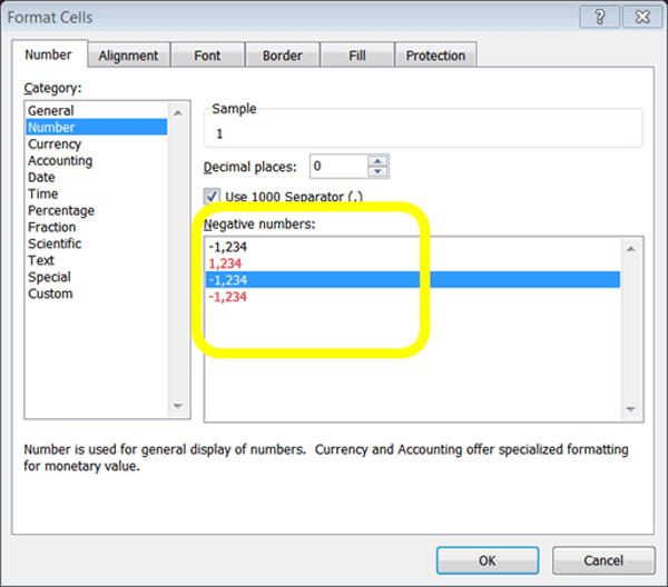
3. In the Negative Numbers box (circled in yellow in the screenshot below), select one of the pre-sets for negative numbers.
4. Press OK to accept the negative number formatting.
Negative numbers will automatically be formatted to the selected type.
* Formatting Dates in Excel – change format of date in Excel
The formatting of dates in Excel is possibly one of the most frustrating issues encountered by users of the program. When typing a date into a cell formatted as a number or currency, for example, Excel will automatically change the date value into a seemingly random number. This can be annoying when all you want is to be able to quickly capture specific dates.
Excel automatically converts a date value that is not formatted as a date to a numerical value. Interestingly, the value that replaces the date you type, for example if you type 15 February 1995 in a cell that is formatted as a Number it will be replaced by the value: 34745, actually means it is that many days since 1 January 1900. If you insert 1 January 1900 into a cell formatted as a number, it will display as 1. Although it may be fun informing your colleagues, friends or family how many days it has been since they were born, it is likely that when you enter a date into Excel, you wish it to display as a date.
To format date values to display as dates:
1. Select the cells, rows or columns you wish to apply the date formatting to.
2. Under the Home tab, in the Number group, click on the Number Format dropdown list.
3. From the list select either Long Date or Short Date. Long Date will display as, for example, 15 February 2015 and short date will display as, for example, 15/02/2015.
What if neither the Long Date nor the Short Date options match the date formatting you require?
1. Click on the Format Cells dialogue box launcher in the right-hand bottom corner of the Number group.
2. Under the Number tab, select Date in the Category box.
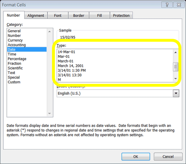
3. Select a date option from the Date Type box (circled in yellow in the screenshot below):
4. Click OK to accept the format change.
TIP: A quick way of inserting the current date into a spreadsheet is by holding down Ctrl on the keyboard whilst pressing the semicolon (;).
* Formatting Fractions in Excel
When it comes to fractions, Excel does all the hard work for you. Instead of spending quality time with your calculator trying to work out how to convert a number such as 0.523523, for example, into a fraction, use the fraction formatting option in Excel.
1. Select the cells, rows or columns to format as fractions.
2. Under the Home tab in the Number group, select Fraction from the Number Format dropdown list.
3. Your selected cells will automatically be converted into fractions.
You can find more fraction formatting options by launching the Format Cells dialogue box by clicking the dialogue box launcher in the right-hand corner of the Number group.
1. In the Format Cells dialogue box, ensure the Number tab is selected and then click on Fractions in the Category list.
2. From the Type box select the fraction type you require your numbers to be formatted as.
3. Press OK to accept the change.
Go ahead and experiment with the different numbering formats covered in this tutorial. Study their effect on different number types and even experiment with the other numbering formats available from the Category box in the Format Cells dialogue box. Remember: practice makes perfect!
Woohoo! Now that you have done the tutorial:
Test your Excel skills with the corresponding FREE Online Multiple Choice
Formatting Numbers Excel Test
TRY THE NEXT TUTORIAL: Understanding Excel Functions Tutorial
TRY THE NEXT TEST: Understanding Excel Functions Test


