Formulas in Excel – Functions in Excel
Basic Excel Formulas Tutorial

Excel 2010 Tutorial – Formulas & Functions
Free Online Microsoft Excel Tutorial

* Understanding Cell References in Excel
* Add in Excel – SUM Function in Excel – Adding Values in Excel
* Subtract in Excel – Subtracting Values in Excel
* Multiply in Excel – Multiply Values – Divide in Excel – Divide Values

Powerful and dynamic arithmetic formulas and functions differentiate Excel from simply, for example, using a table in a Word document or a sheet of paper to list number values. A good place to start is with getting to know how cell references work. Experiment with getting Excel to work for you by learning how to use the Add, Subtract, Multiply, Divide, SUM and AutoSum formulas and functions.

Test your Excel skills with the corresponding FREE Online Multiple Choice
Formulas in Excel – Functions in Excel Basic – Excel Formulas Test

* Understanding Cell References in Excel

The letter and number combinations that make up cell references in Excel may appear a difficult and daunting aspect to master.  These references hold the key to understanding functions and formulas in Excel and are definitely worth familiarizing yourself with.

One way of understanding cell references is to view them as cell addresses.  Each cell reference refers to a specific cell in an Excel Worksheet.  Excel is divided into rows and columns that form a grid.  Rows are numbered 1, 2, 3 onwards and columns are labelled A, B, C onwards.  Each cell on the grid will therefore fall within a specific column and row.

For example, in the screenshot below, the selected cell (which has been highlighted in yellow to make it easier to identify) falls within column D and row 7:

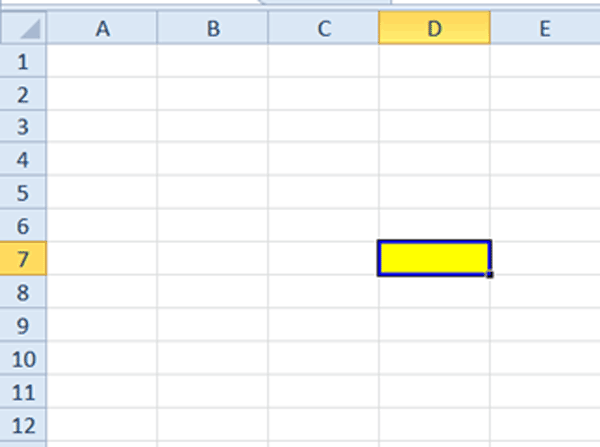
Instead of writing out the above reference as column D, row 7, in Excel we simply state the reference is: D7.

Study the screenshot below.  Can you identify the cell reference for the yellow highlighted cell?

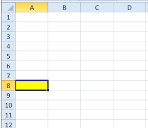
If your answer is A8 that is absolutely correct!  The highlighted cell falls in the column labelled A and the row number 8.

A quick way to read the cell reference for the cell your cursor is positioned in is to use the Name Box (circled in yellow in the screenshot below) located in the top left corner above the column labels:

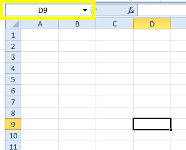
In the screenshot example above it is clear that the cell reference is D9.

Excel also makes provision for cell references comprising multiple cells that are selected at the same time, for example, numbers that are listed in column A and rows 1, 2, 3, 4 and 5.  Study the screenshot of this example below:

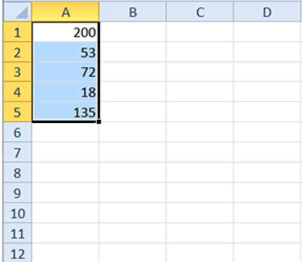
A cell reference such as the one in the screenshot above is written as A1:A5, which means column A and row 1 to column A and row 5 is selected.  The colon between A1 and A5 replaces the word to. 

Study the screenshot below and see if you can identify the cell reference for the selected cells:

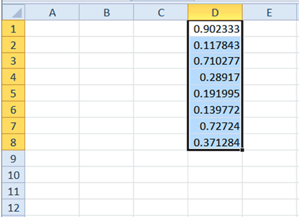
In the example above, the cell reference would be D1:D8, which means that cells in column D and rows 1 to 8 are selected.

The cell reference for cells that are not adjacent to one another are indicated by placing each individual reference or range separated by a comma.  For example,  A1, D2-D9, L3

* Add in Excel – SUM Function in Excel – Adding Values in Excel

Excel is a very powerful calculation tool.  You can use it to create simple budgets, expense sheets or any other type of project where you need a dynamic system of adding values together, calculating the difference between dates, balancing debits and credits to complex scientific calculations.  The most basic calculation, which is a great place to start your Excel journey, is to use the SUM function to add together two or more numbers.

There are a couple of different methods to use the built in SUM function in Excel.  To see this function in action, do the following:

1.  Open a blank worksheet in Excel.

2.  Insert any number values in cells A1 to A4, for example, 250, 300, 500 and 651.

3.  Select cells A1 to A4.

4.  Under the Home tab on the Ribbon click on the AutoSum button (circled in yellow in the screenshot below) in Editing Group.  (You can also access the AutoSum button by clicking on the Formulas tab and accessing it from the Function Library group.

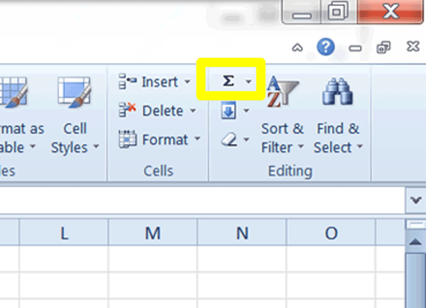
5. Press the Enter key on your keyboard to accept the formula.

6  Excel will AutoSum your selected values and display the total in the first empty cell below your selected cells (in our example A5). 

8.  If you click in the cell that contains your total (A5), you will be able to see the formula that AutoSum automatically inserted by studying the Formula Bar (circled in yellow in the screenshot below).

 

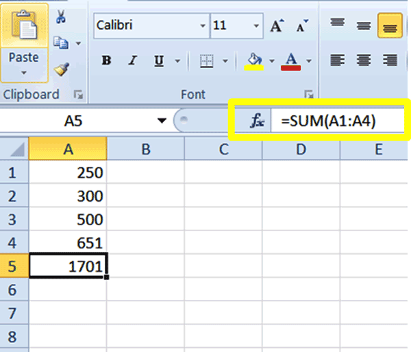
If we deconstruct the formula (circled in yellow in the screenshot above), it simply means the selected cell (A5) equals the sum of the values contained in cells A1 to A4.

1.  To create this formula manually, delete the contents of the cell containing the total (in our example A5).

2.  Position your cursor in the cell you wish to display your total in and type: =Sum(A1:A4)

3.  After you press enter to accept the formula, the calculation total will be displayed in the cell (A5).

The above two methods will work if the numbers you wish to sum are located in adjacent cells in the same column or row.  What happens if you need to sum values that are contained in non-adjacent cells or values that are not even on the same worksheet?

Study the screenshot below:

 

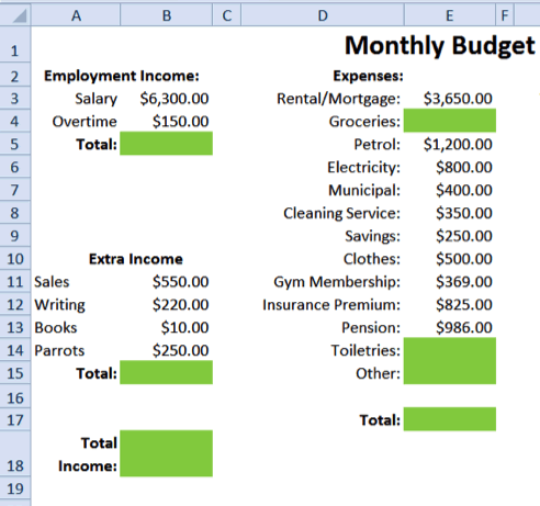
The creator of the above worksheet needs to add together multiple non-adjacent values in order to get specific values.  Using the AutoSum method will not work as this method will add up numbers that are directly adjacent to each other in a row or column.  Entering the Sum formula manually will require that each cell reference and range be inserted in the formula, for example:  =Sum(B5, B15), entered in cell B18 in the example screenshot above, will give the total income value.

Manually entering references may be cumbersome and could lead to errors when the wrong references are inadvertently included in a formula.

A quick way to sum non-adjacent cells is to:

1.  Use a blank worksheet and enter values in random different (and non-adjacent) cells, columns and rows.

2.  Select the cell you wish to display the sum total in and type:  =Sum(

3.  Hold down the Ctrl key on your keyboard and use your left mouse button to select all the cells which contain values you wish to add to the total. 

4.  Once you have selected all the cells you wish to add to the formula, release the Ctrl key and press the Enter key to accept the formula.

You can use the above method to select combinations of rows, columns, non-adjacent cells and even make selections on separation worksheets.

* Subtract in Excel – Subtracting Values in Excel

To subtract values from one another:

1.  Select the cell in which you want the calculation result to appear in.

2.  Type the equal sign:  =

3.  Type the cell reference of the cell that contains the first value (you can also click in the cell that contains this value directly).

4.  Type the minus symbol: –

5.  Type the cell reference of the cell containing the value you wish to subtract from the first value (you can also click in the cell that contains this value directly).

6.  Press enter to accept the formula and display the result of the calculation.

Study the screenshot below.  How would the formula to subtract the Total Expenditure (E17) value from the Total Income (B18) value look if entered into cell D22 (highlighted in green)?

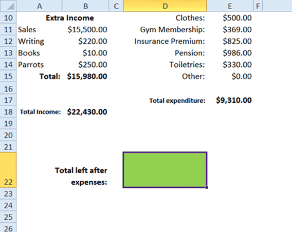
The formula entered into D22 to subtract the expenditure from the income value would be:  =B18-E17

* Multiply in Excel – Multiply Values – Divide in Excel – Divide Values

Once you have mastered using Excel to Sum and Subtract values for you, the next step is mastering multiplication and division of cell values. You may, for example, have an invoice where you need to calculate how much to pay someone for working 10 hours at $24 or need to divide values to get the cost value of a single unit in a box.

In Excel the symbol for multiplication is the asterisk (*).  To divide values we use the division symbol (/).

To experiment with multiplying numbers:

1.  Open a blank worksheet.

2.  In cell A1 type the number 10.

3.  In cell B1 type 25.

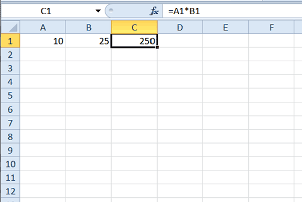
4.  Position your cursor in cell C1 and type the following formula:  =A1*B1

5.  Remember, you can also click on cell A1 and B1 respectively to include them in the formula.

6.  Press the Enter key on your keyboard to accept the formula. 

Below is a screenshot of what your completed formula should look like.  Cell C1 displays the result of the calculation and clicking on C1 will display the formula in the Formula Bar:

To create a formula for dividing values:

1.  In the worksheet used for the above example, type 250 in cell A2.

2.  Type 10 in cell B2.

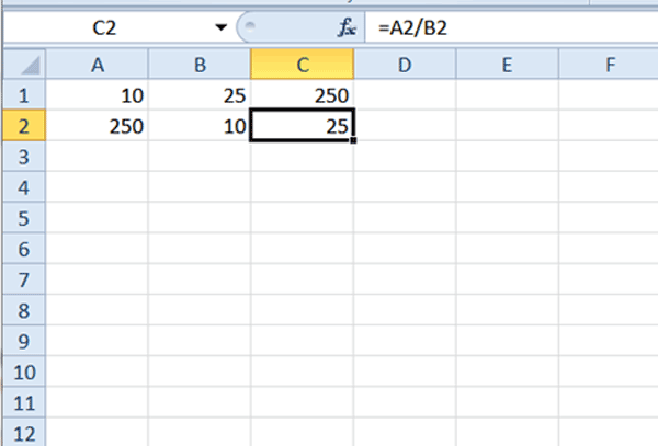
3.  Position your cursor in cell C1 and type the following formula:  =A2/B2.

4.  Remember, you can also click on cell A1 and B1 respectively to include them in the formula.

5. Press the Enter key to accept the formula. 

Below is a screenshot of what your completed formula should look like.  Cell C2 displays the results of the calculation and clicking on the cell will display the formula in the Formula Bar:

Practice entering formulas to sum, subtract, multiply and divide multiple values in rows and columns. Mastering the basics of formulas will ensure that you are able to use ever more complex formulas to automate your worksheets in the future.

Woohoo! Now that you have done the tutorial:

Test your Excel skills with the corresponding FREE Online Multiple Choice
Formulas in Excel – Functions in Excel – Basic Excel Formulas Test

TRY THE NEXT TUTORIAL: Copying Formulas in Excel & Using Relative & Absolute Cell References

TRY THE NEXT TEST: Copying Formulas in Excel & Using Relative & Absolute Cell References Test

* More from Tests Tests Tests.com