www.TestsTestsTests.com
Excel Basics Tutorial
Free Online Microsoft Excel Tutorials
Excel 2010
– Getting Started
* Parts of The Screen
* Columns – Rows – Cells
* Parts of the Worksheet
If you are just starting out in Excel it’s important to identify and understand all the elements that you see on the screen. This includes the Ribbon, Tabs, the Quick Access Toolbar, the Name Box, the Formula Bar, Column and Row Labels, cells and cell addresses and the Worksheet Tabs.
Test your Excel skills with the corresponding FREE Online Multiple Choice
Excel Basics Test
* Parts Of The Screen
This is possibly the most important tutorial in Excel you could invest time in. Knowing the layout of the Excel window will enable you to quickly find functions and make it easier to work out how to complete tasks in Excel. Imagine you are starting a new job, the first few days on the job you will probably spend all your time just learning the layout of the office, who works there and what their functions are. Imagine jumping straight into complex work without even knowing where the lunchroom or bathroom is! It is the same for the Excel screen.
Open Excel and carefully examine the different parts of the screen:

You will note the name of the workbook displayed right at the top, in the middle of the screen. In the example above the name of the workbook is: Book 2 – Microsoft Excel. After you save your workbook, the name you saved it as will appear in this space.
To the right of the workbook title you will note three shapes: a minus symbol, a square and a cross. To minimise the Excel screen so that it becomes ‘minimised’ you press the minus symbol. To ‘maximise’ the screen to a full screen size, you press the square. And to close Excel, you press the cross. These buttons are circled in blue in the image below:

Parallel to the workbook name in the left-hand corner, you will note more or less six icons (circled in blue in the image below). These are shortcuts to functions that people may often use in Excel. This ‘shortcut area’ is called the Quick Access Toolbar or QAT for short. You are able to modify this toolbar by adding more functions or removing functions from it.

In the example above, the buttons displayed are: save (allows you to save a workbook), undo, redo, new (to open a new workbook), open (to open an existing workbook) and quick print.
You are able to customize which buttons you wish to appear on the QAT. To do this press the down pointing arrow located on the right-hand side of the QAT. A list will appear containing functions, some of which will be preceded by a tick mark and some of which are not marked. Those with a tick mark already appear on the QAT. If you wish to remove them use your mouse to click on the function. This will ‘untick’ them and remove the button from the QAT. If you wish to add any of the options that are not on the QAT, simply click on them in the list to add them.

Below the QAT you will observe an area of the screen that appears overrun by function buttons and words. This area is called the Ribbon and it is the ‘control panel’ of any MS Office programme:

The thought of memorising where each function is located may seem a little daunting at first, but luckily for us, the lovely people at Microsoft had a system in mind when organising the Ribbon:
1. The Ribbon is divided into different sections which each contain functions that are related to the name of that section. Sections can be accessed by pressing the section tab above the Ribbon and are named: Home, Insert, Page Layout, Formulas, Data, Review, View and Developer (although this last tab may or may not be enabled on your version of Excel).
You are encouraged to experiment by pressing each tab and studying the type of functions that are available within each section and how they relate to the name of the section (tab).
For example, the Home tab contains all the basic and frequently used functions like formatting, copying and pasting, find and replace etc.
If you click on the Formulas tab, you will find a number of different functions relating to inserting and working with Formulas.
On the Insert tab, you will discover elements that can be inserted into a spreadsheet, like pictures, graphs and tables.
The Page Layout tab allows you to set-up your page type and size, set margins and print areas.
The Data tab offers functions for working with and analysing data in Excel and gives you options to sort or filter data.
The Review tab, like the name says, allows you to review your document using spellchecking, track changes and comments.
Finally, the View tab lets you change how the Excel window is displayed on your screen and different view types offer specific functions that are related to that view.
2. Each section (tab) on the Ribbon is also subdivided into named groups. Click on the Home tab and carefully study this section of the Ribbon:

In the example above, four of the group names have been circled in blue. If you explore the Ribbon you will find that each tab contains different groups. These group names are intended as a collective name for the type of buttons (or functions) you will find in that group. For example, in the group named Font, you find buttons to change the font type, size, colour and other elements related to that group. In the Alignment group, you will find functions to set how data will be aligned on your spreadsheet.
When you need to locate a function in Excel, first think what type of function it is in relation to the tabs on the Ribbon, and once you have identified which tab it belongs to, match it to the appropriate group contained under that tab. This will enable you to quickly find a function!
* Columns, Rows And Cells
Excel is divided into rows, columns and cells and like a game of Battleship, each cell has a place on the grid that can be referenced using the row and column labels.

1. The labels at the top of the sheet are the column labels. These are numbered A, B, C etc all the way to XFD, which admittedly represents more columns than most normal Excel users will ever use!
2. If you study the image below, you will note that columns A, B and D all contain data but that columns C, E, F, G and H are blank:

3. The labels on the left-hand side of the screen represent row numbers in Excel. Numbers start at 1 and go all the way through to 1,048,576, which again represents more rows than anyone would possibly ever get to use!
4. In the image above, rows 1 to 5 contain data, but rows 6 to 12 are all blank.
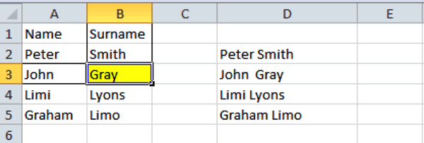
Each block on the grid in Excel represents an individual cell. Cells are referenced by indicating in which column they are located and which row. For example, in the image below, the highlighted cell is located in column B and row 3. The reference or cell address will therefore be B3.

Let’s examine another example. In the image below, the reference or the cell address of the highlighted cell is D5. It is located in column D, row 5:

*
Parts of the Worksheet
The worksheet is the area where the magic really happens, where you add, organise and edit your data. It includes the worksheet tabs, formula bar and the data grid. Imagine it as your data ‘factory’ – it is where the work gets produced, stored, viewed, shared and managed. There may be all sorts of functions going on in the background, but this is where your end product will be visible.
A workbook in Excel is a collective name. Similar to a real book, a workbook may contain one continuous chapter or many chapters. In Excel we call these ‘chapters’ worksheets. By default a workbook opens with three blank worksheets.
1. You will find these displayed as tabs in the bottom left hand corner of the screen. In the example below, these are titled: Sheet1, Sheet2 and Sheet3.

2. If you click on any of these worksheet tabs, it will open a completely different worksheet containing separate sets of data. For example, you may add your budget for each month of the year to a separate sheet or any other data that relates to the same subject that you may want to keep grouped together in one file or workbook.
The Formula Bar is located above the grid (the middle area of your worksheet). It is the blank line prefixed with the letters fx. This is called the Don’t be fooled by its name, it is not solely for the purpose of entering formulas and is also not the only place you can enter a formula into Excel.
1. Study the image below paying attention to the Formula bar (circled in blue):

2. When you add data to Excel, the contents of the selected cell will appear in the formula bar. Study the example below noting the word Peter that is displayed in the selected cell (the cell with a thick black border around it) as well as in the formula bar:

3. Instead of typing straight into a cell, you can type data into the formula bar and the data will be added to the cell you have selected in Excel.
4. The most popular function of the Formula bar is to create formulas and insert functions. Very complex formulas may contain references to multiple worksheets or even workbooks and it is much easier to keep track whilst creating these, by using the Formula bar.
5. The fx located to the left of the Formula bar is a shortcut button to the Insert Function dialogue box which allows you to choose formulas and functions, recently used formulas and functions and gives a short explanation of what each selected formula or function achieves.
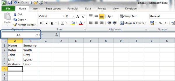
Another essential part of the worksheet to be aware of is the Name Box which you will find just to the left of the Formula Bar.
1. Study the image below taking note of the location of the Name Box (circled in blue):

2. The Name Box is used to add and view the name of a specific selected cell or a group of cells. In the example above the selected cell is A6 and that is the name displayed in the Name Box.
3. The Name Box can also be used to give a specific name to a cell or a group of cells. In the example below, the Name Box displays the name that was given to cells A1 to A5:

4. The Name Box allows you to give a single logical name to multiple sections of data and makes it much easier to construct formulas. If you are viewing a Worksheet that was created by someone else, names for specific sets of data may make the data easier to interpret.
Woohoo! Now that you have done the tutorial:
Test your Excel skills with the corresponding FREE Online Multiple Choice
Excel Basics Test
TRY THE NEXT TUTORIAL:
Using the File Tab in Excel Tutorial
TRY THE NEXT TEST: Using the File Tab in Excel Test


