www.TestsTestsTests.com
Working with Images & Graphical Elements Excel Tutorial
Excel 2010 Training –
Graphical Elements
Free Online Microsoft Excel Tutorial
* How to Insert an Image
*
How to Insert Shapes
* Working with SmartArt
* Changing the Background Color
Just because a worksheet contains a lot of numbers or data does not mean it cannot look good. You can insert images and shapes, background colors and use SmartArt to make a worksheet in Excel visually more appealing.
Test your Excel skills with the corresponding FREE Online Multiple Choice
Working with Images & Graphical Elements Excel Test
* How to Insert an Image
The option to insert images such as company logos, clipart and photos into a worksheet makes it possible to create visually appealing and professional looking workbooks. Applications for this could be, for example, a company invoice requiring a logo, price lists requiring product images or any worksheet that just needs a splash of color and design.
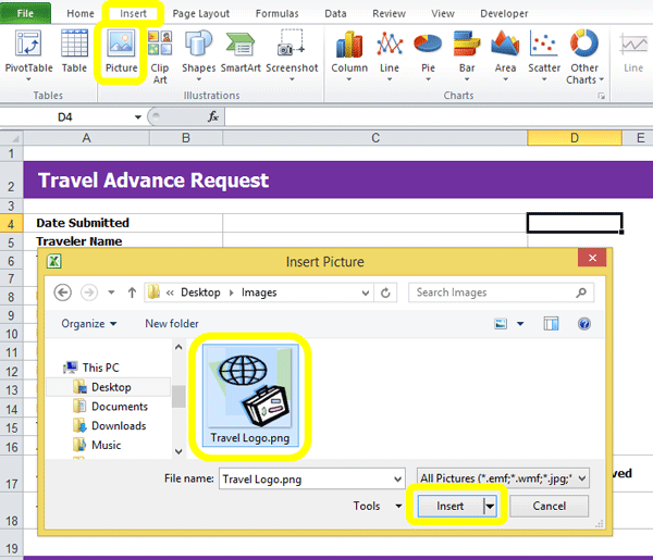
To insert an image into a worksheet:
1. Select the cell or cell area where you wish to insert the image.
2. Click on the Insert tab on the Ribbon.
3. In the Illustrations group, click on Picture. This will open the Windows Explorer box.
4. Navigate to where the image you wish to insert is located and click on the image to select it.
5. Click on the Insert button to close the dialog box. The image will now be available within the worksheet.
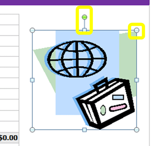
You can resize by clicking on it and dragging the corner markers (circled in yellow to increase or decrease the image size. Use the Green handle to rotate the image by clicking and dragging it to the left or right.
To apply special formatting to your graphic, select any of the available formatting tools under the Format contextual tab. This tab will only be visible when the image is selected. There are options to change the color, add a border, create special effects and countless more options available on this menu. They are definitely worth experimenting with before you turn to your image editing software.
* How to Insert Shapes
There are multiple uses for shapes in a worksheet: you can use it to create a simple diagram, to emphasize content by inserting it in a shape or even use it to create an image.
To insert a shape in a worksheet:
1. Click on the Insert tab on the Ribbon.
2. In the Illustrations group, click on the Shapes button. This will launch the Shape gallery (circled in yellow in the screenshot below):
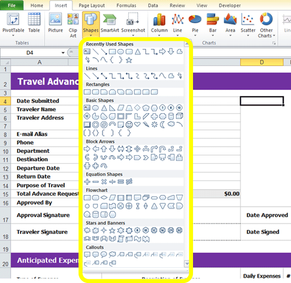
3. Select the shape you wish to insert by clicking on it in the gallery (circled in yellow in the screenshot above).
4. The gallery will close and you can now insert the shape into the worksheet. Click and drag to insert the chosen shape.
You can resize the shape by clicking on the any of the corner handles. Rotate the shape by dragging the green handle to the left or right.
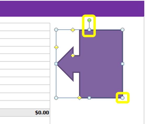
The Drawing Tools contextual tab, which is only available when the shape is selected, provides countless options to format, apply styles and coloring, special effects and other elements to the shape you inserted.
* Working with SmartArt
SmartArt is the clever older brother of shapes. It combines all the functionality and look of shape with an easy to use text box for adding bullets and images to your shapes. It also allows you to organize shapes and select from a gallery of very professional SmartArt diagrams.
To insert SmartArt:
1. Click on the Insert tab on the Ribbon.
2. In the Illustrations group, click on SmartArt. This will launch the SmartArt Graphic gallery:
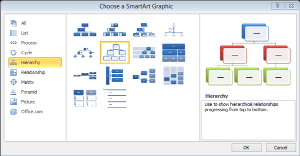
3. Use the list on the left-hand side of the gallery to open a category of SmartArt diagrams. In the example above, the Hierarchy category is selected and 14 pre-designed SmartArt diagrams are available to choose from.
4. When you click on a SmartArt image it will be displayed in the box on the right-hand side together with some information about the image. Click on the OK button to insert the SmartArt diagram into the worksheet.
To add text to a SmartArt diagram:
1. Select the diagram and then click on the arrows to the left of the diagram to open the SmartArt textbox.
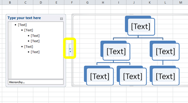
2. In the SmartArt textbox (circled in yellow in the screenshot below), type the text you wish to appear within the SmartArt shapes at different levels. You can also type into the shapes directly, but using the textbox is often an easier option to do this. In addition, if you use the textbox, you can press the Enter key to add more shapes to the SmartArt diagram.
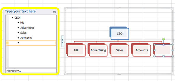
3. You can close the textbox at any time and reopen it by pressing the arrow to the left-hand side of the SmartArt diagram.
Use the SmartArt Tools contextual tabs, which include a Design and Format gallery, to change the look and feel of the diagram. The options are limitless and are worth experimenting with.
You can change the SmartArt diagram at any time without reinserting a new one:
1. Select the SmartArt diagram to change.
2. Click on the Design tab under the SmartArt Tools contextual tab.
3. In the Layouts group, press the gallery button (circled in yellow in the screenshot below) to expand the Layouts gallery.
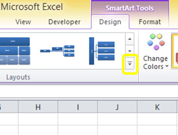
4. Select a different layout. Your SmartArt, including text, will be reformatted into the new diagram.
* Changing the Background Color
A worksheet does not have to have the usual white background. You can change the background color for a whole worksheet and even use an image to set the background.
To change a worksheet background color:
1. Click on the Select All button in the top left-hand corner of the worksheet (circled in yellow in the screenshot below):
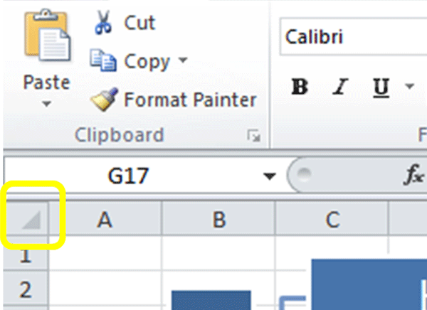
2. In the Font group under the Home tab, click on the dropdown arrow next to the Fill color button.
3. From the Fill Color Gallery, select a color for the worksheet background by clicking on it.
The color will be applied to the entire worksheet.
To insert a background image into a worksheet:
1. Click on the Page Layout tab on the Ribbon.
2. In the Page Setup group, click on Background. This will launch the Windows Explorer dialog box. Find the image you wish to insert into the background and click on the Insert button.
The selected image will be tiled in the background of the worksheet. To remove it, simply click on the Remove Background button in the Page Setup group.


