
www.TestsTestsTests.com

Customizing Number &
Text Formats in Excel Tutorial
Excel 2016 Tutorial
Data Entry and Formatting in Excel 2016
Free Online Microsoft Excel Tutorials
* Currency Format in Excel – Accounting Formats in Excel 2016
* Decimal Places & Percentage Format in Excel – How to add percentage in Excel
* Date Format in Excel – Time Format in Excel 2016
* How to use Custom Formats Excel 2016
|
Excel treats all data entered in the form of text or numbers in a specific way depending on whether it is a numerical value, percentage, text, date, time, currency, etc. |
 |
* Currency Format in Excel – Accounting Formats in Excel 2016
The default format for text and numbers typed into cells in a worksheet in Excel is General. However, if you are working with currency values you can apply the Currency Format to the cell so that it is automatically formatted with the selected currency symbol. Applying the currency format also tells Excel that the contents of the cell is a monetary value and to treat it as such.
In the example screenshot below, the column outlined in orange contains monetary values (Cost).
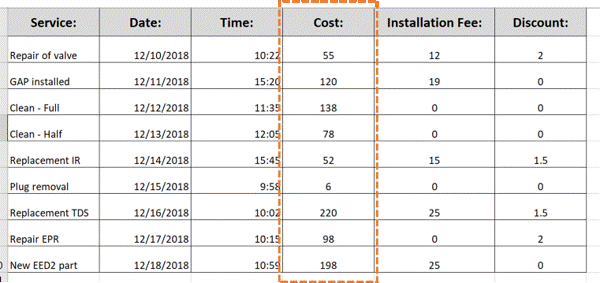
Instead of typing the dollar symbol ahead of each transaction value, you can use the Currency or Accounting Number Formats
To apply the Currency Format:
1. Select the cell(s), column(s) or row(s) containing the values you want to format as a currency.
2. Under the Home tab on the Ribbon, in the Number group, click on the dropdown arrow next to the Number Format box, outlined in orange in the screenshot below:
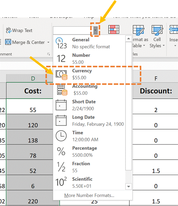
3. Select Currency from the dropdown list (outlined in orange in the screenshot above) to apply the default currency your computer system is set to, to the selected cells. In the screenshot above the default currency is $.
To select a different currency:
1. Click on More Number Formats at the bottom of the Number Format list.
2. In the Currency category select the currency symbol you are looking for from the Symbol list and click OK to apply.
TIP: Use the shortcut key combination: Ctrl + Shift + $ to apply the Currency Format.
You can also apply the Accounting Number Format, which inserts the currency symbol but also formats the numbers into an accounting format with the currency symbol aligned to the left of the cell and the values aligned to the right.
To apply the Accounting Number Format:
1. Select the cell(s), column(s) or row(s) containing the values you want to format using the Accounting style.
2. Under the Home tab on the Ribbon, in the Number group, click on the Accounting Number Formatbutton to apply this format or click the dropdown arrow next to the button and select one of the other accounting formats to apply.
* Decimal Places & Percentage Format in Excel – How to add percentage in Excel
Numerical values entered into cells can automatically be formatted with the percentage symbol and a pre-set number of decimal places.
To create pre-formatted cells that will automatically add a % symbol to the end of a value, do the following:
1. Select the cell(s), column(s) or row(s) where you want to insert percentage values.
2. Under the Home tab on the Ribbon, in the Number group click on the Percentage button. This will apply the format to your cell selection. When you type a number value into one of the formatted cells, the percentage symbol will appear.
Applying the Percentage Format to existing values may require you to use a formula to convert the values to percentages, for example, division of the value by 100 and then applying the Percentage Format to the result.
TIP: Use the keyboard shortcut combination Ctrl + Shift + % to apply the Percentage Format.
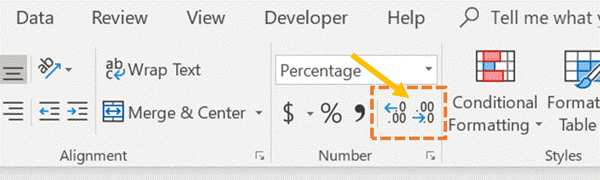
Working with decimals in Excel is super easy! Click the Increase Decimal or Decrease Decimal buttons to instantly reduce/increase the number of decimals in a value.
You will find the Decimal Format options under the Home tab on the Ribbon in the Number group (outlined in orange in the screenshot below):
* Date Format in Excel – Time Format in Excel 2016
Using the correct Date and Time formats in Excel is essential not only for making the data display correctly but also to make formulas work as intended.
There are several built in Date formats and you can even customize how you want a date to display. Later versions of Excel, like Excel 2016 for Office 365, recognizes and automatically formats a value that looks like a date. For example, if you type 1 Dec 2018, Excel will automatically change the number format from General to Custom (date).
To apply date formats:
1. Select the cell(s), column(s) or row(s) you want to format.
2. Under the Home tab on the Ribbon, in the Numbers group, click the down pointing arrow for the Number Format menu.
3. Select one of the pre-set date formats: short date or long date to apply to your selection.
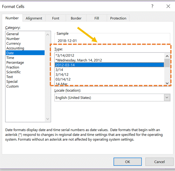
To customize the Date Format:
1. Select More Number Formats from the Number Format menu. This will launch the Format Cells dialog box.
2. Select the Date category and pick one of the Custom Date formats in the Type box (see screenshot below):
3. Press OK to apply the date format to your selection.
TIP 1: You can format dates according to your location, for example, applying standard date display formats for the United States or Britain.
TIP 2: Use the keyboard shortcut combination Ctrl + Shift + # to apply the date format.
Time Formats work in much the same way as Date Formats do. Apply a specific Time Format by following these steps:
1. Select the cell(s), column(s) or row(s) you want to format.
2. Under the Home tab on the Ribbon, in the Numbers group, click the down pointing arrow for the Number Format menu.
3. Select the Time Format option from the menu list by clicking on it.
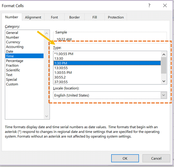
To customize the Time Format:
1. Select More Number Formats from the Number Format menu. This will launch the Format Cells dialog box.
2. Select the Time category and pick one of the custom time formats in the Type box (see screenshot below):
3. Press OK to apply the Time Format to your selection.
TIP: Use the keyboard shortcut combination: Ctrl + Shift + @ to apply the Time Format to cells.
* How to use Custom Formats Excel 2016
You can customize how the contents of a cell is formatted by creating Custom formats in Excel. These can range from very simple to highly complex number formatting codes.
To experiment with Custom formats:
1. Select the cell(s), row(s) or column(s) you want to create a Custom format for.
2. Under the Home tab on the Ribbon, in the Number Format group, click the dropdown arrow next to the Number Format box.
3. Select More Number Formats from the Number Format menu.
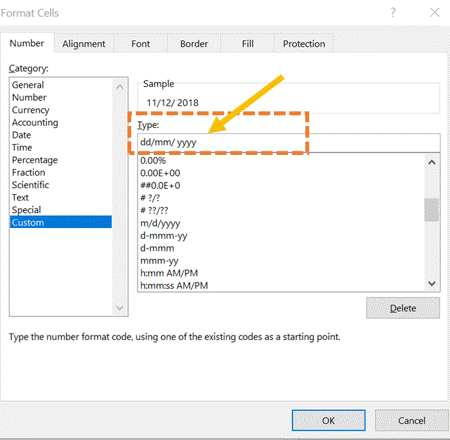
4. In the Format Cells dialog box, click on Custom.
5. In the Type box, select one of the Custom formats that most resemble the format you are looking for, for example d-mmm-yy, will display a date as 11-Dec-18
6. Use the Type box to modify the formatting code to a format that fits your needs (see outlined in orange in the screenshot below), for example, dd/mm/yyyy will display a date as 11/12/2018. The Sample box above the Type box will show you what the format will look like when applied.
7. Press OK to apply the Custom Format you selected/created.
To remove any number formats applied to cells:
1. Select the cells
2. Under the Home tab in the Number group, click the Number Format dropdown arrow and select General at the top of the menu list.
Experiment with building your own custom number format codes. Comprehensive lists of codes for number formats can be found on Microsoft Excel and Office 365 websites.
Woohoo! Now that you have done the tutorial:
Test your Excel skills with the corresponding FREE Online Multiple Choice
Customizing Number & Text Formats in Excel 2016 – Data Entry and Formatting
* TRY THE NEXT TEST: How to Add Excel Borders & Shading to Cells Test
* TRY THE NEXT TUTORIAL: How to Add Excel Borders & Shading to Cells Tutorial